
The SRC(L) framework
Every graph pooling operator can be expressed through a framework called SRC (Select, Reduce, Connect), introduced in the paper Understanding Pooling in Graph Neural Networks. The SRC framework is a powerful abstraction that allows you to define graph pooling operators in a modular way. In particular, a generic graph pooling operator is given by the composition of three functions: Select (\(\texttt{SEL}\)), Reduce (\(\texttt{RED}\)), and Connect (\(\texttt{CON}\)). Let’s say that our original graph has \(N\) nodes and the node features of these nodes are stored in a set \(\mathcal{X}\). Similarly, the graph has \(E\) edges and the edge features are in a set \(\mathcal{E}\). In the example below, the original graph has \(N=5\) nodes and \(E=5\) edges. Let’s also say that the pooled graph has \(K\) supernodes with features \(\mathcal{X}'\), while the edge features are stored in a set \(\mathcal{E}'\). In the example, the pooled graph has 3 supernodes and 2 edges.

Even if it is not part of the original framework, there is an additional operation called \(\texttt{LIFT}\), which is used to map the pooled node features \(\mathcal{X}'\) back to the original node space. This is used in architectures with an AutoEncoder structure to solve tasks at the node level (e.g., node classification/regression) or at the edge level (e.g., link prediction).

Every pooling operator in  tgp is implemented according to the SRC(L) framework.
Select
The \(\texttt{SEL}\) function is responsible for deciding how many supernodes the pooled graph will have and which nodes of the original graph will end up in which supernode. In other words, \(\texttt{SEL}\) determines which nodes are selected and how they are grouped together. Note that \(\texttt{SEL}\) can also select only a subset of all nodes and discard the others. The \(\texttt{SEL}\) function is arguably the most important part of a pooling method. In fact, the specific implementation of \(\texttt{SEL}\) is what mostly sets different pooling methods apart.
For example, a cluster-based pooler groups the \(N\) nodes into \(K\) clusters, which become the supernodes of the pooled graph. In this case, we can view the \(\texttt{SEL}\) operation as a soft-clustering assignment matrix \(\mathbf{S}\) that maps each node to its cluster with a given membership value.
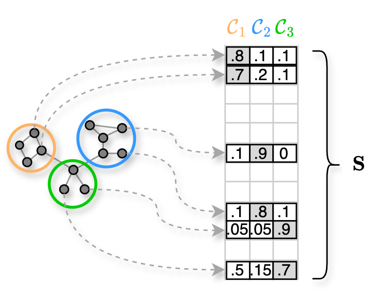
It turns out that the output of any \(\texttt{SEL}\) operation can be expressed with a similar matrix. For example, we can think of the output of a 1-over-\(K\) pooling method that selects a subset of the nodes of the original graph as a matrix \(\mathbf{S}\) with 1 in correspondence of selected nodes, and 0 for nodes that are dropped.
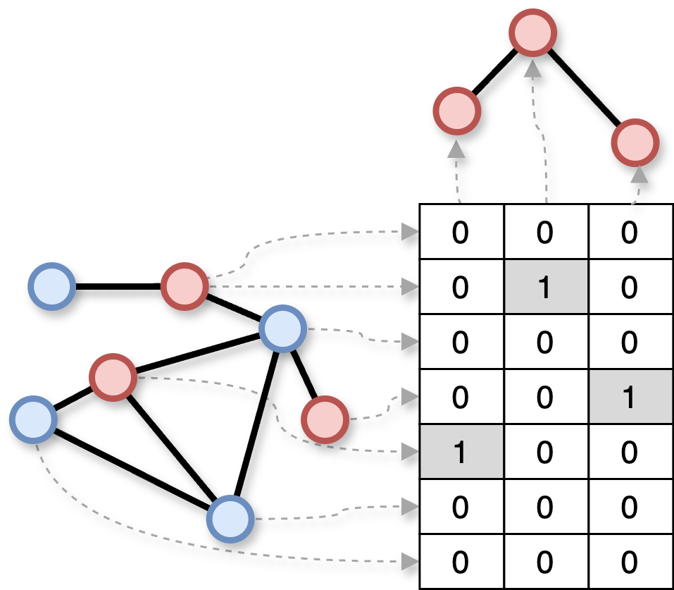
Similarly, for a scoring-based method such as Top-\(K\), the select matrix will contain non-zero entries for the nodes that are kept and 0 for those that are dropped. In addition, the non-zero entries will have a value equal to the top-\(K\) scores associated with selected nodes.
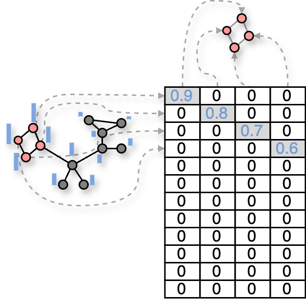
In tgp, the \(\mathbf{S}\) matrix is contained within the object SelectOutput, along with other useful information to perform pooling.
Reduce
The \(\texttt{RED}\) operation is responsible for computing the node features of the pooled graph. Each pooling method can implement the \(\texttt{RED}\) function differently, but in general the result depends on the topology, the node (and edge) features of the original graph, and the output of the \(\texttt{SEL}\) function.
Let’s make a practical example and let’s say that \(\texttt{RED}\) computes the features \(\mathbf{X}' \in \mathbb{R}^{K, \cdot}\) by taking the sum, the max, or the average of the features \(\mathbf{X} \in \mathbb{R}^{N, \cdot}\) that are assigned by \(\texttt{SEL}\) to the same supernode. In matrix form, we can express this \(\texttt{RED}\) operation simply as:
Connect
The \(\texttt{CON}\) function is similar in spirit to \(\texttt{RED}\), except that it deals with the edges and the edge features of the pooled graph. In particular, \(\texttt{CON}\) decides how the nodes of the pooled graph are connected and what ends up in the edge features of the pooled graph. As for \(\texttt{RED}\), the output of \(\texttt{CON}\) depends on the original graph and, clearly, also on \(\mathbf{S}\), the output of \(\texttt{SEL}\).
For example, let’s say that the \(\texttt{CON}\) operation creates an edge \(e_{ij}\) between supernodes \(i\) and \(j\) by summing all edges whose endpoints are assigned to \(i\) and \(j\), respectively. When the aggregation operation is the sum, like in this example, we can express the \(\texttt{CON}\) operation in matrix notation:
where \(\mathbf{A}' \in \mathbb{R}^{K \times K}\) is the adjacency matrix of the pooled graph.
Lift
The purpose of \(\texttt{LIFT}\) is to map the pooled node features \(\mathbf{X}' \in \mathbb{R}^{K, \cdot}\) back to the original space. In other words, the lifted features \(\mathbf{\tilde X} \in \mathbb{R}^{N, \cdot}\) and the original features \(\mathbf{X} \in \mathbb{R}^{N, \cdot}\) have the same node dimension \(N\). We can think of \(\texttt{LIFT}\) as the operation that “undoes” \(\texttt{RED}\):
The most principled way of implementing \(\texttt{LIFT}\) is by applying to the pooled node features the pseudo-inverse of the selection matrix:
In practice it might be enough to just use \(\mathbf{S}\) to lift the features, which is faster as it avoids inverting the matrix: