Advanced details

In the following, we will analyze in more details the pooler operators, see how their components interact, and what differs from one operator to the others.

If you’re running this in Google Colab, you might need to restart the session after running the installation cell below.

import sys
if 'google.colab' in sys.modules:
    %pip install torch==2.4.1 --index-url https://download.pytorch.org/whl/cu124
    %pip install torch_geometric==2.6.1
    %pip install torch_scatter torch_sparse torch_cluster -f https://data.pyg.org/whl/torch-2.4.0+cu124.html
    %pip install pygsp==0.6.1
    %pip install -q git+https://github.com/tgp-team/torch-geometric-pool.git@main

Let’s start by importing the required libraries.

import torch
import matplotlib.pyplot as plt
import networkx as nx
from torch_geometric.data import Batch, Data
from torch_geometric.datasets import TUDataset
from torch_geometric.loader import DataLoader
from torch_geometric.nn import NNConv
from torch_geometric.utils import to_networkx

from tgp.connect import DenseConnect, KronConnect, SparseConnect
from tgp.datasets import PyGSPDataset
from tgp.lift import BaseLift
from tgp.poolers import MinCutPooling, NDPPooling, TopkPooling
from tgp.reduce import AggrReduce, GlobalReduce, get_aggr
from tgp.select import TopkSelect

torch.manual_seed(42)
torch.set_printoptions(threshold=3, edgeitems=3)

Matplotlib is building the font cache; this may take a moment.

We will consider three pooling methods:

• TopkPooling, a sparse pooling method with trainable parameters;

• NDPPooling, a sparse pooling method without trainable parameters that precomputes the node assignments and the poole graph;

• MinCutPooling, a dense pooling method with trainable parameters and auxiliary losses.

Before looking at the pooling operators in detail, let’s first load some data.

dataset = TUDataset(root="/tmp/MUTAG", name="MUTAG")
print(f"Dataset: {dataset}")
loader = DataLoader(dataset, batch_size=3, shuffle=True)
data_batch = next(iter(loader))
print(f"Data batch: {data_batch}")

Downloading https://www.chrsmrrs.com/graphkerneldatasets/MUTAG.zip

Dataset: MUTAG(188)
Data batch: DataBatch(edge_index=[2, 94], x=[44, 7], edge_attr=[94, 4], y=[3], batch=[44], ptr=[4])

Processing...
Done!

The dataset contains edge attributes, i.e., vectors associated with each edge of the graph. The pooling operators in tgp assume that the edge attributes are already embedded into the node features by a MP layers before pooling. For the complete list of MP that support edge attributes refer to the GNN cheatsheet. A simple MP layer that does the job is NNConv.

adj = data_batch.edge_index
batch = data_batch.batch
feat_size = 16

# Embed the node and edge features into new features
x = NNConv(
    in_channels=dataset.num_features,
    out_channels=feat_size,
    nn=torch.nn.Linear(dataset.num_edge_features, dataset.num_features * feat_size),
)(data_batch.x, adj, data_batch.edge_attr)

The edge features are now embedded into the node features x.

Let’s now look at the pooling operators and their output.

# Instantiate the pooler
topk = TopkPooling(in_channels=feat_size)
print(topk)

# Compute the pooling output
topk_out = topk(x=x, adj=adj, batch=batch)
print(topk_out)

TopkPooling(
	select=TopkSelect(in_channels=16, ratio=0.5, act=Tanh(), s_inv_op=transpose)
	reduce=BaseReduce()
	lift=BaseLift(matrix_op=precomputed, reduce_op=sum)
	connect=SparseConnect(reduce_op=sum, remove_self_loops=True, edge_weight_norm=False, degree_norm=False)
	multiplier=1.0
)
PoolingOutput(so=[44, 23], x=[23, 16], edge_index=[2, 42], edge_weight=None, batch=[23], mask=None, loss=None)

# Instantiate the pooler
ndp = NDPPooling()
print(ndp)

# Compute the pooling output
ndp_out = ndp(x=x, adj=adj, batch=batch)
print(ndp_out)

NDPPooling(
	select=NDPSelect(s_inv_op=transpose)
	reduce=BaseReduce()
	lift=BaseLift(matrix_op=precomputed, reduce_op=sum)
	connect=KronConnect(sparse_threshold=0.01)
	cached=False
)
PoolingOutput(so=[44, 19], x=[19, 16], edge_index=[2, 60], edge_weight=[60], batch=[19], mask=None, loss=None)

# Instantiate the pooler
mincut = MinCutPooling(
    in_channels=feat_size, k=dataset._data.num_nodes // len(dataset) // 2
)
print(mincut)

# Compute the pooling output
mincut_out = mincut(x=x, adj=adj, batch=batch)
print(mincut_out)

MinCutPooling(
	select=MLPSelect(in_channels=[16], k=8, act=None, dropout=0.0, s_inv_op=transpose)
	reduce=BaseReduce()
	lift=BaseLift(matrix_op=precomputed, reduce_op=sum)
	connect=DenseConnect(remove_self_loops=True, degree_norm=True, adj_transpose=True, edge_weight_norm=False, sparse_output=False)
	batched=True
	cut_loss_coeff=1.0
	ortho_loss_coeff=1.0
)
PoolingOutput(so=[20, 8], x=[3, 8, 16], edge_index=[3, 8, 8], edge_weight=None, batch=None, mask=[3, 8], loss=['cut_loss', 'ortho_loss'])

A few things to keep in mind:

• Almost every method share the same \(\texttt{RED}\) and \(\texttt{LIFT}\) operators.

• The \(\texttt{SEL}\) operator is what sets most methods apart and, besides a few exceptions (e.g., NMFSelect) Dense poolers use the same \(\texttt{SEL}\) operation.

• Finally, \(\texttt{CON}\) is usually implemented by SparseConnect or DenseConnect, depending if the method is dense or sparse. However, there are a few exceptions such as NDPPooling that uses KronConnect.

Select

The \(\texttt{SEL}\) operator computes the assignment of the nodes to the supernodes of the pooled graph. The output of the \(\texttt{SEL}\) operator is stored inside the SelectOutput.

The general signature of the \(\texttt{SEL}\) operator is the following.

so_topk = topk.select(
    x=x, edge_index=adj, edge_weight=None, batch=batch, num_nodes=x.shape[0]
)
print(so_topk)

SelectOutput(num_nodes=44, num_supernodes=23)

Not all arguments are used by a given pooling method. For example, TopkSelect requires only the node features x and batch to perform pooling.

so_topk = topk.select(
    x=x,
    batch=batch,
)
print(so_topk)

SelectOutput(num_nodes=44, num_supernodes=23)

SelectOutput

The SelectOutput has several fields. The first and most important is s, which is the select matrix \(\mathbf{S} \in \mathbb{R}^{N \times K}\). In the case of a sparse pooler, s is a torch.sparse.Tensor (COO format) representing \(\mathbf{S}\in\mathbb{R}^{N\times K}\).

print(f"s type: {type(so_topk.s)}")
print(f"shape: {so_topk.s.shape}")
print(f"is_sparse: {so_topk.s.is_sparse}")

s type: <class 'torch.Tensor'>
shape: torch.Size([44, 23])
is_sparse: True

The content of \(\mathbf{S}\) can be accessed by the following properties of the SelectOutput.

print(
    f"node index: {so_topk.node_index}\n"
    f"cluster_index: {so_topk.cluster_index}\n"
    f"weight: {so_topk.weight}\n"
)

node index: tensor([ 0,  1,  2,  ..., 36, 37, 38])
cluster_index: tensor([ 4,  3,  0,  ..., 17, 22, 18])
weight: tensor([0.8031, 0.8031, 0.8213,  ..., 0.8213, 0.8031, 0.8177],
       grad_fn=<ValuesBackward0>)

Note

Note that we have gradients in weight. In TopkPooling such weights allow for the gradients to pass through the non-differentiable top-\(k\) operation.

Another important field of the SelectOutput is \(\mathbf{S}_\text{inv}\), which is used by the \(\texttt{LIFT}\) operation.

so_topk.s_inv

tensor(indices=tensor([[ 4,  3,  0,  ..., 17, 22, 18],
                       [ 0,  1,  2,  ..., 36, 37, 38]]),
       values=tensor([0.8031, 0.8031, 0.8213,  ..., 0.8213, 0.8031, 0.8177]),
       size=(23, 44), nnz=23, layout=torch.sparse_coo, grad_fn=<TBackward0>)

By default, we s_inv is the transpose of s, i.e, \(\mathbf{S}_\text{inv} = \mathbf{S}^\top\). However, we can also use the pseudo-inverse, \(\mathbf{S}_\text{inv} = \mathbf{S}^+\).

so_topk_pinv = TopkSelect(in_channels=dataset.num_features, s_inv_op="inverse")(
    x=data_batch.x, batch=data_batch.batch
)
print(so_topk_pinv.s_inv)

tensor(indices=tensor([[ 0,  1,  2,  ..., 20, 21, 22],
                       [ 6,  9, 12,  ..., 33, 34, 35]]),
       values=tensor([ 3.0269,  3.0269,  3.0269,  ..., 24.8659, 24.8659,
                      24.8659]),
       size=(23, 44), nnz=23, layout=torch.sparse_coo,
       grad_fn=<ToSparseBackward1>)

Hint

We can specify how to compute \(\mathbf{S}_\text{inv}\) by setting either s_inv_op="transpose" or s_inv_op="inverse" when we instantiate the pooler.

There are a few other properites accessible from the SelectOutput. In particular, we check whether the pooling operator is expressive or not, according to the expressivity conditions.

print(
    f"num_nodes: {so_topk.num_nodes}\n"
    f"num_supernodes: {so_topk.num_supernodes}\n"
    f"expressive: {so_topk.is_expressive}\n"
)

num_nodes: 44
num_supernodes: 23
expressive: False

Sparse methods are generally not expressive, while dense methods are.

# Sparse select
so_ndp = ndp.select(
    edge_index=adj,
)
print(f"expressive: {so_ndp.is_expressive}\n")

expressive: False

# Dense select
so_mincut = mincut.select(
    x=x,
)
print(f"expressive: {so_mincut.is_expressive}\n")

expressive: True

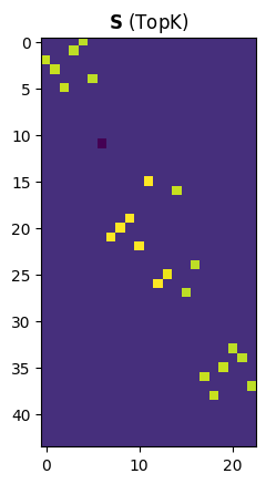
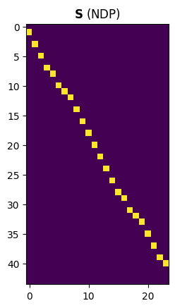
Generally, the select matrix \(\mathbf{S}\) of a sparse method is a sparse matrix with one non-zero entry for each row, meaning that each node is assigned to only one supernode.

plt.imshow(so_topk.s.to_dense().detach().numpy(), cmap="viridis")
plt.title(r"$\mathbf{S}$ (TopK)");

plt.imshow(so_ndp.s.to_dense().detach().numpy(), cmap="viridis")
plt.title(r"$\mathbf{S}$ (NDP)");

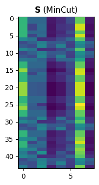
In dense methods such as MinCutPool, \(\mathbf{S}\in\mathbb{R}^{B \times N \times K}\) is a dense soft cluster assignment matrix, usually computed directly from the node features \(\mathbf{X}\) as:

\[\mathbf{S} = \mathrm{softmax}\big(\texttt{MLP}(\mathbf{X})\big).\]

print(f"so_mincut.s: {so_mincut.s.shape}")

so_mincut.s: torch.Size([1, 44, 8])

In the dense case, all the elements \(\mathbf{S}\) are generally non-zero.

fig, ax = plt.subplots(figsize=(2, 4))
ax.imshow(
    so_mincut.s.detach().numpy().reshape(-1, so_mincut.num_supernodes),
    cmap="viridis",
    aspect="auto",
)
plt.title(r"$\mathbf{S}$ (MinCut)");

Reduce

The \(\texttt{RED}\) operation determines how to compute the node features of the pooled graph \(\mathbf{X}_\text{pool} \in \mathbb{R}^{K \times F}\) from the features \(\mathbf{X} \in \mathbb{R}^{N \times F}\) of the original graph, given the SelectOutput.

x_pool_topk, batch_pool_topk = topk.reduce(x=x, so=so_topk, batch=batch)
print(x_pool_topk.shape)

torch.Size([23, 16])

In practice, \(\texttt{RED}\) computes the features of each supernode \(i\) by aggregating the features of each node \(i\) assigned to \(j\). For example, when the aggregation is the sum, we have:

\[ \mathbf{X}_\text{pool}[i] = \sum_j \mathbf{S}_\text{inv}[j,i] \cdot \mathbf{X}[j]. \]

In general, we can use other types of aggregation, such as "mean", "max", etc…

mean_reduce = AggrReduce(get_aggr("mean"))
x_pool_mean, _ = mean_reduce(x, so_topk, batch=batch)
print(x_pool_mean.shape)

torch.Size([23, 16])

AggrReduce wraps PyG’s Aggregation operators: any torch_geometric.nn.aggr aggregator can be used for the REDUCE step. Use string names via get_aggr("mean"), get_aggr("max"), or parametrized ones like get_aggr("lstm", in_channels=..., out_channels=...), and pass the result to AggrReduce(aggr) or to GlobalReduce(reduce_op=aggr). For global readout, instantiate GlobalReduce(reduce_op="sum"|"mean"|...) once (e.g. in __init__) and call it on node features; reduce_op can be a string or a PyG Aggregation instance.

# Other aggregations: pass a PyG Aggregation (e.g. via get_aggr) to AggrReduce or GlobalReduce
max_reduce = AggrReduce(get_aggr("max"))
x_pool_max, _ = max_reduce(x, so_topk, batch=batch)
# Same aggregators work in GlobalReduce(..., reduce_op="mean"|"sum"|aggr_instance)

In the case of dense methods, the \(\texttt{RED}\) operation does not require to provide the batch indexes, as the batch dimension is explicit in the first dimension of x_dense.

x_pool_mc, batch_pool_mc = mincut.reduce(x=x, so=so_mincut)
print(x_pool_mc.shape)

torch.Size([1, 8, 16])

Global reduce

Global reduce is the operation that aggregates all the nodes of a graph into a single output. This can be thought as a special case of \(\texttt{RED}\), where all the nodes are aissgned to a single supernode and is often referred to as global pooling in the GNN literature.

Attention

The global pooling operation is called global reduce in tgp.

The aggreation operations used in global reduce are the same as the standard reduce, i.e., "sum", "mean", "min", etc…

reducer_glob_sparse = GlobalReduce(reduce_op="sum")
x_pool_glob = reducer_glob_sparse(x_pool_topk, batch=batch_pool_topk)
print(x_pool_glob.shape)

torch.Size([3, 16])

For dense methods the same GlobalReduce infers format from the tensor shape (3D). Also in this case, the batch is explicit in the first dimension and we do not need to pass the batch indices.

reducer_glob_dense = GlobalReduce(reduce_op="sum")
x_pool_glob_dense = reducer_glob_dense(
    x_pool_mc, batch=None
)  # we do not pass batch here
print(x_pool_glob_dense.shape)

torch.Size([1, 16])

Note that GlobalReduce returns the same shape for both sparse (2D input) and dense (3D input) tensors.

Connect

Given the original connectivity matrix \(\mathbf{A}\) and the SelectOutput, the \(\texttt{CON}\) operation is responsible to generate the connectivity matrix of the pooled graph \(\mathbf{A}_\text{pool}\).

For sparse methods, SparseConnect returns a list of edges representing the edges of the pooled graphs in the batch.

ei_pool_topk, ew_pool_topk = topk.connect(
    edge_index=adj, edge_weight=data_batch.edge_weight, so=so_topk
)
print(f"A_pool (topk): {ei_pool_topk.shape}")

A_pool (topk): torch.Size([2, 42])

Sparse methods like TopkPooling that implements the \(\texttt{CON}\) operation with SparseConnect allow to specify different types of aggregations for the edges. The default is "sum", which leads to the following computation of the connectivity matrix:

\[ \mathbf{A}_\text{pool} = \mathbf{S}^\top \mathbf{A} \mathbf{S}_\text{inv}. \]

Also in this case, other operations can be used to aggregate the edges by setting, e.g., reduce_op="mean" or reduce_op="min". Additionally, the \(\mathbf{A}_\text{pool}\) might contain self loops that can be removed by setting the correspondent flag.

sp_conn = SparseConnect(reduce_op="mean", remove_self_loops=True)
ei_pool_topk, ew_pool_topk = sp_conn(
    edge_index=adj, edge_weight=data_batch.edge_weight, so=so_topk
)
print(f"A_pool (topk): {ei_pool_topk.shape}")

A_pool (topk): torch.Size([2, 42])

Hint

We can specify how to aggregate the edges by, e.g., setting connect_red_op="sum" or connect_red_op="mean" when we instantiate the pooler.

Some particular methods like NDPPooling use a special \(\texttt{CON}\) operation, KronConnect, which behaves differently and does not offer the same options of SparseConnect.

ei_pool_ndp, ew_pool_ndp = ndp.connect(
    edge_index=adj, edge_weight=data_batch.edge_weight, so=so_ndp
)
print(f"A_pool (ndp): {ei_pool_ndp.shape}")

A_pool (ndp): torch.Size([2, 74])

Or equivalently:

kron_conn = KronConnect()
ei_pool_ndp, ew_pool_ndp = kron_conn(
    edge_index=adj, edge_weight=data_batch.edge_weight, so=so_ndp
)
print(f"A_pool (ndp): {ei_pool_ndp.shape}")

A_pool (ndp): torch.Size([2, 74])

The dense methods use their own \(\texttt{CON}\) method, DenseConnect, which returns a dense tensor of shape \([B, K, K]\). If remove_self_loops = True the diagonal of \(\mathbf{A}_\text{pool}\) is set to zero, while degree_norm = True applies a symmetric degree-normalization and returns \(\mathbf{\tilde A}_\text{pool} = \mathbf{D}^{-1/2}_\text{pool} \mathbf{A}_\text{pool} \mathbf{D}^{-1/2}_\text{pool}\).

dense_conn = DenseConnect(remove_self_loops=True, degree_norm=True)
adj_pool_mc, _ = dense_conn(adj, so_mincut)
print(f"A_pool (mincut): {adj_pool_mc.shape}")

A_pool (mincut): torch.Size([1, 8, 8])

Lift

The \(\texttt{LIFT}\) operation maps the pooled node features \(\mathbf{X}_\text{pool} \in \mathbb{R}^{K \times F}\) back to the original node space \(\mathbf{X}_\text{lift} \in \mathbb{R}^{N \times F}\). The \(\texttt{LIFT}\) operation is implemented as:

\[ {X}_\text{lift} = \mathbf{S}_\text{inv} \mathbf{X}_\text{pool}. \]

x_lift_topk = topk.lift(x_pool=x_pool_topk, so=so_topk)
print(f"x (original): {x.shape}")
print(f"x_pool (topk): {x_pool_topk.shape}")
print(f"x_lift (topk): {x_lift_topk.shape}")

x (original): torch.Size([44, 16])
x_pool (topk): torch.Size([23, 16])
x_lift (topk): torch.Size([44, 16])

Also in this case, the default aggregation is "sum", but we can specify other aggregation types by setting, e.g., reduce_op="mean". We can also specify if we want to lift using \(\mathbf{S}_\text{inv} = \mathbf{S}^\top\), \(\mathbf{S}_\text{inv} = \mathbf{S}^+\), or just using the value currently stored in SelectOutput.s_inv by setting matrix_op="transpose", matrix_op="inverse", or matrix_op="precomputed", respectively.

lifter = BaseLift(reduce_op="mean", matrix_op="inverse")
x_lift_topk = lifter(x_pool=x_pool_topk, so=so_topk)
print(f"x_lift (topk): {x_lift_topk.shape}")

x_lift (topk): torch.Size([44, 16])

Hint

We can specify the lift aggregation and the \(\mathbf{S}_\text{inv}\) to be used by passing the desired values to the lift_red_op and lift variables of the pooler, respectively.

The same lifter can also be used for dense pooling operators.

x_lift_mc = lifter(x_pool=x_pool_mc, so=so_mincut)
print(f"x (dense): {x.shape}")
print(f"x_pool (mincut): {x_pool_mc.shape}")
print(f"x_lift (mincut): {x_lift_mc.shape}")

x (dense): torch.Size([44, 16])
x_pool (mincut): torch.Size([1, 8, 16])
x_lift (mincut): torch.Size([1, 44, 16])

Combining and reusing existing operators

The existing implementations of the \(\texttt{SEL}\), \(\texttt{RED}\), \(\texttt{CONN}\), and \(\texttt{LIFT}\) operators can be combined in several ways and re-used when building new pooling methods.

For example, one could replace the connector of TopkPooling with KronConnect.

# Instantiate the pooler and replace the connector
topk_kron = TopkPooling(in_channels=feat_size, ratio=0.5)
topk_kron.connector = KronConnect()
print(topk_kron)

# Compute the pooling output
topk_kron_out = topk_kron(x=x, adj=adj, batch=batch)
print(topk_kron_out)

TopkPooling(
	select=TopkSelect(in_channels=16, ratio=0.5, act=Tanh(), s_inv_op=transpose)
	reduce=BaseReduce()
	lift=BaseLift(matrix_op=precomputed, reduce_op=sum)
	connect=KronConnect(sparse_threshold=0.01)
	multiplier=1.0
)
PoolingOutput(so=[44, 23], x=[23, 16], edge_index=[2, 58], edge_weight=[58], batch=[23], mask=None, loss=None)

/home/docs/checkouts/readthedocs.org/user_builds/torch-geometric-pool/checkouts/latest/tgp/connect/kron_conn.py:82: UserWarning: Laplacian not provided. The SelectOutput is not computed with NDPSelect.
  warnings.warn(

In general, when implementing a new sparse pooling operator, it will likely re-use the existing BaseReduce, SparseConnect, and BaseLift functions. Similarly, a dense pooling operator will likely use MLPSelect, BaseReduce, DenseConnect, and BaseLift.

Visualization

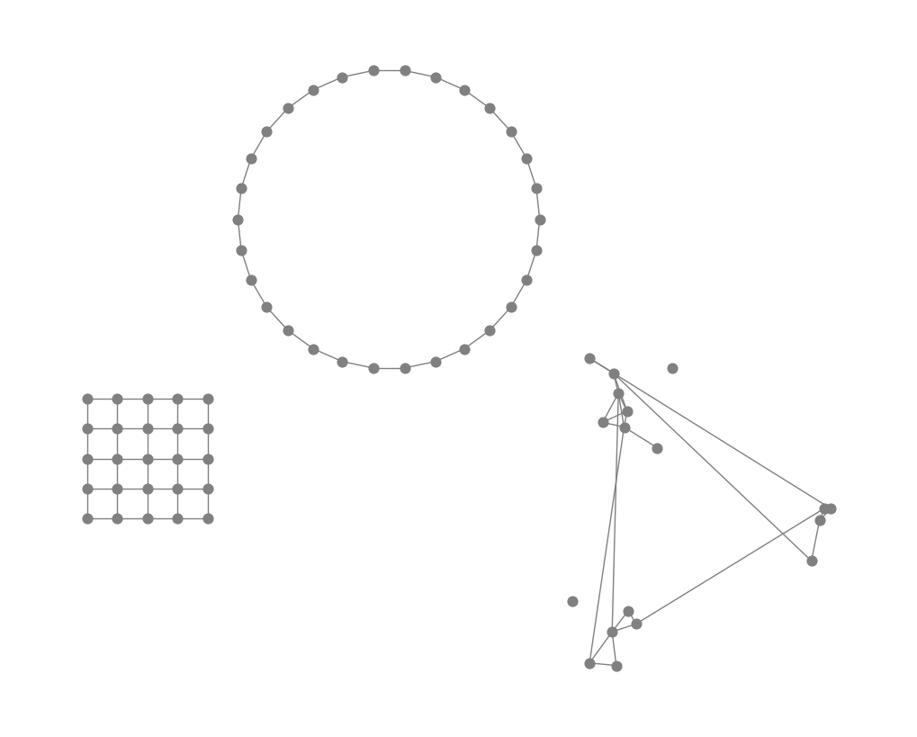
The modular and standardized API of the poolers in tgp allows for using the same functions to visualize the pooling results. For testing and debugging, we can rely on the simple point clouds provided by the PyGSP library for which tgp provide a wrapper for converting them into a proper torch dataset. Below, we create a batch composed of a 2D-Grid, a Ring, and a Community graphs.

grid = PyGSPDataset(
    root="/tmp/PyGSP/",
    name="Grid2d",
    transform=None,
    pre_transform=None,
    pre_filter=None,
    force_reload=True,
    kwargs={"N1": 5, "N2": 5},
)[0]
print(f"2D-Grid: {grid}")

ring = PyGSPDataset(
    root="/tmp/PyGSP/",
    name="Ring",
    transform=None,
    pre_transform=None,
    pre_filter=None,
    force_reload=True,
    kwargs={"N": 30},
)[0]
ring.update({"x": ring.x + 2.0})
print(f"Ring: {ring}")

community = PyGSPDataset(
    root="/tmp/PyGSP/",
    name="Community",
    transform=None,
    pre_transform=None,
    pre_filter=None,
    force_reload=True,
    kwargs={"N": 18, "Nc": 3},
)[0]
community.update(
    {"x": torch.stack([community.x[:, 0] * 0.2 + 4.0, community.x[:, 1] * 0.2], dim=1)}
)
print(f"Community: {community}")

Processing...
Done!
Processing...
Done!
2026-04-21 09:17:25,386:[INFO](pygsp.graphs.community.__init__): Constructed using eps-NN with eps = 1.4564753151219703

2D-Grid: Data(x=[25, 2], edge_index=[2, 80], y=[25], edge_weight=[80])
Ring: Data(x=[30, 2], edge_index=[2, 60], y=[30], edge_weight=[60])
Community: Data(x=[18, 2], edge_index=[2, 50], y=[18], edge_weight=[50])

Processing...
Done!

# Create a batch from the three datasets
pygsp_batch = Batch.from_data_list([grid, ring, community])
print(pygsp_batch)

DataBatch(x=[73, 2], edge_index=[2, 190], y=[73], edge_weight=[190], batch=[73], ptr=[4])

# Plot the batch
G = to_networkx(pygsp_batch, to_undirected=True)
plt.figure(figsize=(10, 8))
nx.draw(
    G, pos=pygsp_batch.x.numpy(), node_size=60, node_color="gray", edge_color="gray"
)

Let’s first consider the NDPPooling, which is a sparse method that is not trained and, as such, can provide a meaningful pooling output without performing any training.

# Instantiate the pooler and compute the output
ndp = NDPPooling()
ndp_out = ndp(x=pygsp_batch.x, adj=pygsp_batch.edge_index, batch=pygsp_batch.batch)

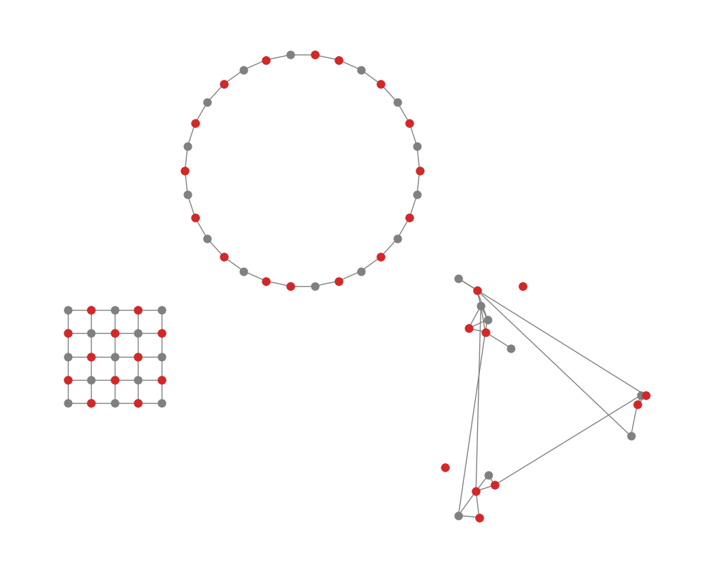
Below, we visualize the outcome of the \(\texttt{SEL}\) operation. NDPPooling selects one-very-other nodes, meaning that we expect to see the selected nodes to be disconnected.

plt.figure(figsize=(10, 8))
nx.draw(
    G, pos=pygsp_batch.x.numpy(), node_size=60, node_color="gray", edge_color="gray"
)

# We plot in different colors the selected nodes
nx.draw_networkx_nodes(
    G,
    pos=pygsp_batch.x.numpy(),
    nodelist=ndp_out.so.node_index,  # selected nodes
    node_color="tab:red",
    node_size=60,
);

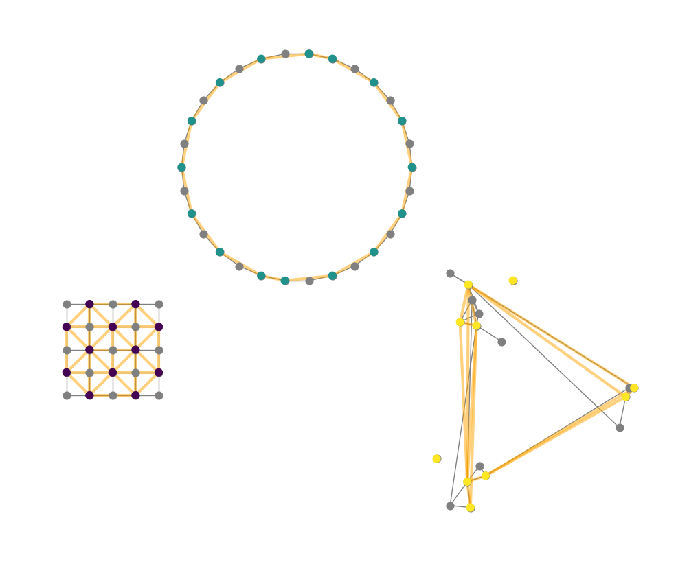
Finally, we can plot \(\mathbf{X}_\text{pool}\) (we use different colors for each graph in the batch) and \(\mathbf{A}_\text{pool}\) (orange edges).

g_pooled = Data(
    x=ndp_out.x, edge_index=ndp_out.edge_index, edge_weight=ndp_out.edge_weight
)
G_pooled = to_networkx(g_pooled, to_undirected=True)

plt.figure(figsize=(10, 8))
nx.draw(
    G, pos=pygsp_batch.x.numpy(), node_size=60, node_color="gray", edge_color="gray"
)
nx.draw_networkx_nodes(
    G_pooled, pos=ndp_out.x.numpy(), node_size=60, node_color=ndp_out.batch
)
nx.draw_networkx_edges(
    G_pooled, pos=ndp_out.x.numpy(), edge_color="orange", width=3, alpha=0.5
);

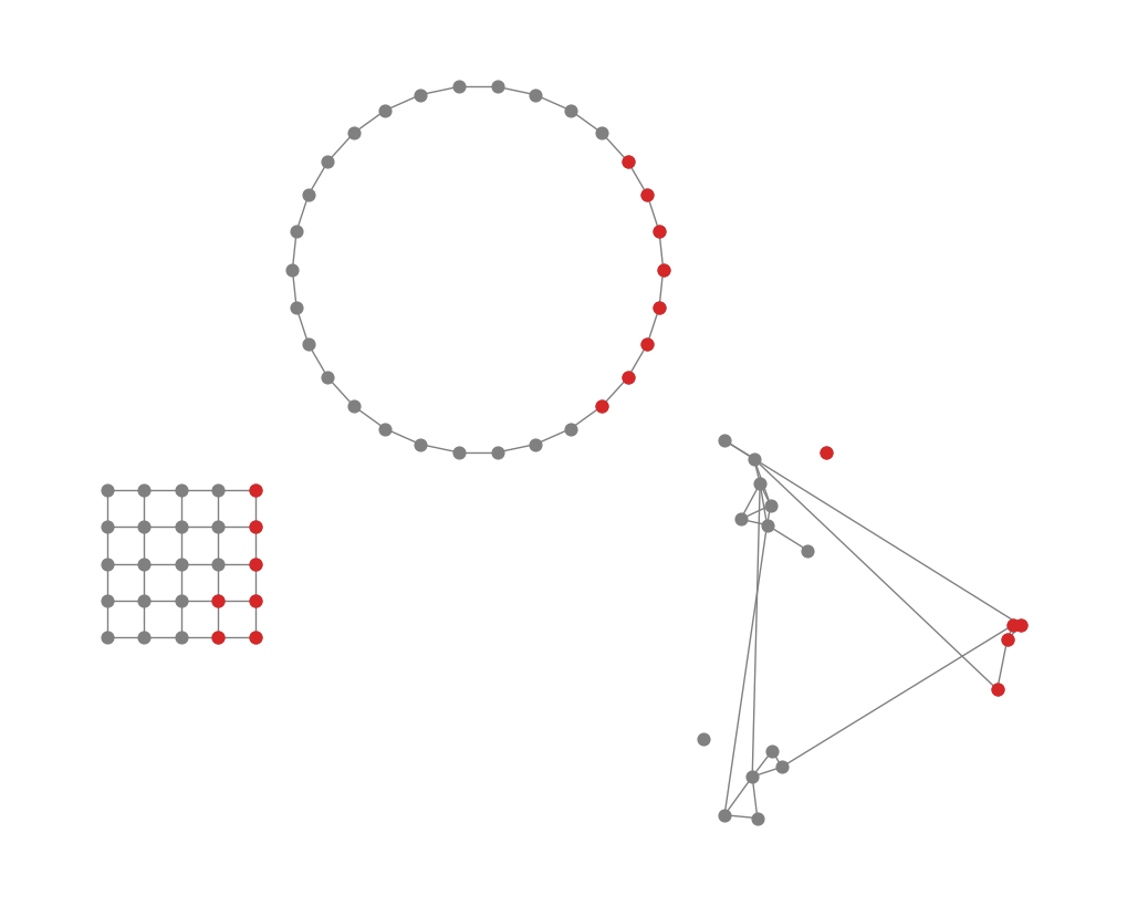
We can use the same procedure to plot the selected nodes of other poolers. For TopkPooling we get the following.

# Instantiate the pooler and compute the output
topk = TopkPooling(in_channels=2, ratio=0.25)
topk_out = topk(x=pygsp_batch.x, adj=pygsp_batch.edge_index, batch=pygsp_batch.batch)

plt.figure(figsize=(10, 8))
nx.draw(
    G, pos=pygsp_batch.x.numpy(), node_size=60, node_color="gray", edge_color="gray"
)

# We plot in different colors the selected nodes
nx.draw_networkx_nodes(
    G,
    pos=pygsp_batch.x.numpy(),
    nodelist=topk_out.so.node_index,  # selected nodes
    node_color="tab:red",
    node_size=60,
);

# Plot the pooled graph
g_pooled = Data(
    x=topk_out.x, edge_index=topk_out.edge_index, edge_weight=topk_out.edge_weight
)
G_pooled = to_networkx(g_pooled, to_undirected=True)

plt.figure(figsize=(10, 8))
nx.draw_networkx_nodes(
    G_pooled, pos=topk_out.x.detach().numpy(), node_size=60, node_color=topk_out.batch
)
nx.draw_networkx_edges(
    G_pooled, pos=topk_out.x.detach().numpy(), edge_color="orange", width=3, alpha=0.5
);

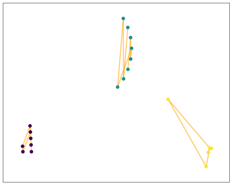
Note that the result in this case does not make much sense because TopkPooling must be trained to produce meaningful results.

Combining existing pieces

One of the most powerful features of tgp is the ability to create custom pooling operators by mixing and matching different \(\texttt{SEL}\), \(\texttt{RED}\), \(\texttt{CON}\), and \(\texttt{LIFT}\) components. You can subclass SRCPooling and pass your own selector, reducer, lifter, and connector.

Available components include Select (e.g. TopkSelect, NDPSelect), Connect (SparseConnect, DenseConnect, KronConnect), Reduce (BaseReduce), and Lift (BaseLift).

Below we implement a custom pooler that combines TopkSelect with KronConnect (instead of the default SparseConnect used by TopkPooling), then use it in a GNN and train on MUTAG.

from tgp.poolers import TopkPooling
from tgp.connect import KronConnect



class CustomTopKKronPooler(TopkPooling):
    """Custom pooler: TopkSelect + BaseReduce + BaseLift + KronConnect (instead of SparseConnect)."""

    def __init__(self, in_channels, ratio=0.5):
        super().__init__(in_channels=in_channels, ratio=ratio)
        self.connector = KronConnect()
        

custom_pooler = CustomTopKKronPooler(in_channels=feat_size, ratio=0.5)
print("Custom pooler:", custom_pooler)
out = custom_pooler(x=x, adj=adj, batch=batch)
print("Output:", out)

Custom pooler: CustomTopKKronPooler(
	select=TopkSelect(in_channels=16, ratio=0.5, act=Tanh(), s_inv_op=transpose)
	reduce=BaseReduce()
	lift=BaseLift(matrix_op=precomputed, reduce_op=sum)
	connect=KronConnect(sparse_threshold=0.01)
	multiplier=1.0
)
Output: PoolingOutput(so=[44, 23], x=[23, 16], edge_index=[2, 56], edge_weight=[56], batch=[23], mask=None, loss=None)

Use the custom pooler in a GNN (conv → pool → conv → global pool → linear) and train on MUTAG:

import torch.nn.functional as F
from torch_geometric.nn import GCNConv, Linear

class GNNWithCustomPooler(torch.nn.Module):
    def __init__(self, hidden_channels=64):
        super().__init__()
        self.conv1 = GCNConv(dataset.num_features, hidden_channels)
        self.pooler = CustomTopKKronPooler(in_channels=hidden_channels, ratio=0.5)
        self.conv2 = GCNConv(hidden_channels, hidden_channels)
        self.lin = Linear(hidden_channels, dataset.num_classes)
        self.readout = GlobalReduce(reduce_op="sum")

    def forward(self, x, edge_index, edge_weight, batch):
        x = self.conv1(x, edge_index, edge_weight)
        x = F.relu(x)
        pool_out = self.pooler(x=x, adj=edge_index, edge_weight=edge_weight, batch=batch)
        x = self.conv2(pool_out.x, pool_out.edge_index, pool_out.edge_weight)
        x = F.relu(x)
        x = self.readout(x, batch=pool_out.batch)
        x = F.dropout(x, p=0.5, training=self.training)
        x = self.lin(x)
        return F.log_softmax(x, dim=-1)


device = torch.device("cuda" if torch.cuda.is_available() else "cpu")
train_loader = DataLoader(dataset[:150], batch_size=32, shuffle=True)
test_loader = DataLoader(dataset[150:], batch_size=32)

model = GNNWithCustomPooler(hidden_channels=64).to(device)
optimizer = torch.optim.Adam(model.parameters(), lr=0.01)


def train():
    model.train()
    total_loss = 0
    for data in train_loader:
        data = data.to(device)
        optimizer.zero_grad()
        out = model(data.x, data.edge_index, data.edge_weight, data.batch)
        loss = F.nll_loss(out, data.y.view(-1))
        loss.backward()
        optimizer.step()
        total_loss += data.num_graphs * float(loss)
    return total_loss / len(train_loader.dataset)


@torch.no_grad()
def test(loader):
    model.eval()
    correct = 0
    for data in loader:
        data = data.to(device)
        pred = model(data.x, data.edge_index, data.edge_weight, data.batch).argmax(dim=-1)
        correct += int(pred.eq(data.y.view(-1)).sum())
    return correct / len(loader.dataset)


for epoch in range(1, 101):
    loss = train()
    if epoch % 20 == 0:
        test_acc = test(test_loader)
        print(f"Epoch {epoch:3d}, Loss: {loss:.4f}, Test Acc: {test_acc:.4f}")
print(f"Final test accuracy: {test(test_loader):.4f}")

Epoch  20, Loss: 0.4954, Test Acc: 0.7105

Epoch  40, Loss: 0.4563, Test Acc: 0.7368

Epoch  60, Loss: 0.4502, Test Acc: 0.8158

Epoch  80, Loss: 0.4268, Test Acc: 0.8158

Epoch 100, Loss: 0.4254, Test Acc: 0.8158
Final test accuracy: 0.8158