Hierarchical Graph Neural Networks with tgp

Graph pooling is a fundamental operation in Graph Neural Networks (GNNs) that enables hierarchical learning by coarsening graphs into smaller representations. Just as convolutional neural networks use pooling to build hierarchical features in images, graph pooling allows GNNs to capture multi-scale patterns in graph-structured data.

In this tutorial, we’ll explore tgp (Torch Geometric Pool), a comprehensive library that provides a unified framework for graph pooling operators. We’ll learn how to:

• Understand the SRC framework (\(\texttt{SEL}\)-\(\texttt{RED}\)-\(\texttt{CON}\)) that unifies all pooling operators

• Visualize pooling operations to understand what they do

• Build GNNs with and without pooling to understand the benefits

• Work with both sparse and dense poolers

• Create hierarchical architectures with multiple pooling layers

• Optimize performance with caching and precoarsening

• Create custom pooling operators by mixing and matching components

For more details, see the tgp paper and the documentation.

Let’s get started!

Setup and Installation

First, let’s install the required libraries. If you’re running this in Google Colab, you might need to restart the session after running the installation cell below.

import sys
if 'google.colab' in sys.modules:
    %pip install torch==2.4.1 --index-url https://download.pytorch.org/whl/cu124
    %pip install torch_geometric==2.6.1
    %pip install torch_scatter torch_sparse torch_cluster -f https://data.pyg.org/whl/torch-2.4.0+cu124.html
    %pip install pygsp==0.6.1
    %pip install -q git+https://github.com/tgp-team/torch-geometric-pool.git@main

Now let’s import the libraries we’ll need throughout this tutorial.

import torch
import torch.nn.functional as F
from torch.nn import Linear
from torch_geometric.data import Batch
from torch_geometric.datasets import TUDataset, Planetoid
from torch_geometric.loader import DataLoader
from torch_geometric.nn import ARMAConv, GCNConv, DenseGCNConv
from torch_geometric import seed_everything
from torch_geometric.utils import to_dense_adj, to_networkx, to_dense_batch

# Visualization imports
import matplotlib.pyplot as plt
import networkx as nx

from tgp.data import PreCoarsening, PoolDataLoader
from tgp.datasets import PyGSPDataset
from tgp.poolers import get_pooler, pooler_classes, pooler_map
from tgp.reduce import BaseReduce, GlobalReduce

# Set random seed for reproducibility
seed_everything(42)
torch.set_printoptions(threshold=2, edgeitems=2)

# Load MUTAG dataset (we'll use this throughout the tutorial)
dataset = TUDataset(root='/tmp/MUTAG', name='MUTAG')

The SRC Framework

All pooling operators in tgp follow the SRC framework, which decomposes pooling into three fundamental operations:

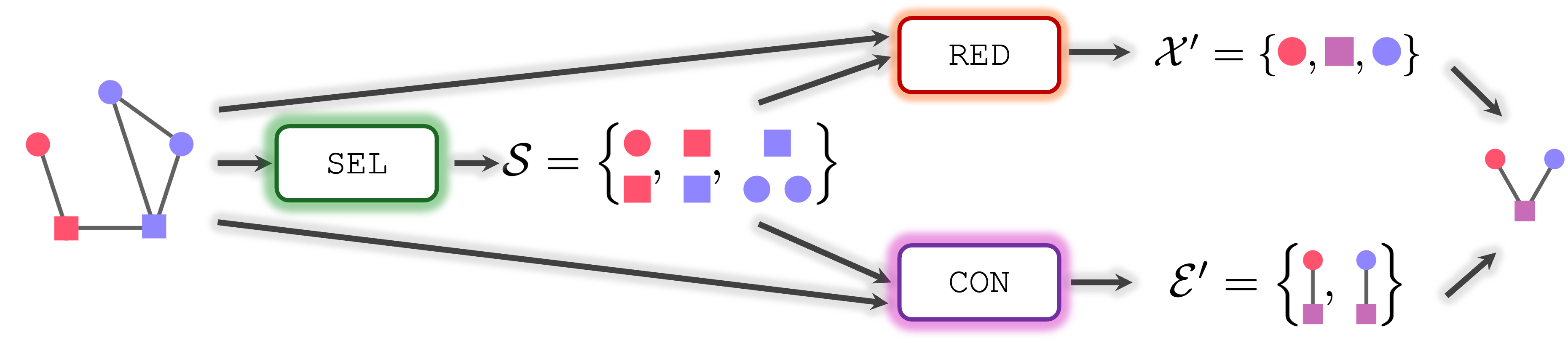
• \(\texttt{SEL}\) (SELECT): Determines how nodes map to supernodes (i.e. the nodes of the coarsened graph). This produces a SelectOutput containing the assignment matrix \(\mathbf{S}\).

• \(\texttt{RED}\) (REDUCE): Aggregates features of nodes assigned to the same supernode using \(\mathbf{S}\).

• \(\texttt{CON}\) (CONNECT): Creates edges between supernodes in the coarsened graph using \(\mathbf{S}\).

There’s also a \(\texttt{LIFT}\) operation for unpooling (mapping coarsened features back to the original graph), which is useful for tasks like node classification.

This abstraction makes it easy to understand, compare, and create custom pooling operators. For more details, see the SRC paper.

Let’s explore the available poolers:

print("Available pooling operators in tgp:")
for i, pooler in enumerate(pooler_classes):
    print(f"{i+1:2d}. {pooler}")

Available pooling operators in tgp:
 1. ASAPooling
 2. AsymCheegerCutPooling
 3. BNPool
 4. DiffPool
 5. DMoNPooling
 6. EdgeContractionPooling
 7. EigenPooling
 8. GraclusPooling
 9. HOSCPooling
10. LaPooling
11. JustBalancePooling
12. KMISPooling
13. MaxCutPooling
14. MinCutPooling
15. NDPPooling
16. NMFPooling
17. NoPool
18. PANPooling
19. SAGPooling
20. SEPPooling
21. TopkPooling

Each pooler has a convenient alias for quick instantiation using get_pooler:

print("Pooler aliases:")
for alias, cls in pooler_map.items():
    print(f"  '{alias:8s}' → {cls.__name__}")

Pooler aliases:
  'asap    ' → ASAPooling
  'acc     ' → AsymCheegerCutPooling
  'bnpool  ' → BNPool
  'diff    ' → DiffPool
  'dmon    ' → DMoNPooling
  'ec      ' → EdgeContractionPooling
  'eigen   ' → EigenPooling
  'graclus ' → GraclusPooling
  'hosc    ' → HOSCPooling
  'lap     ' → LaPooling
  'jb      ' → JustBalancePooling
  'kmis    ' → KMISPooling
  'maxcut  ' → MaxCutPooling
  'mincut  ' → MinCutPooling
  'ndp     ' → NDPPooling
  'nmf     ' → NMFPooling
  'nopool  ' → NoPool
  'pan     ' → PANPooling
  'sag     ' → SAGPooling
  'sep     ' → SEPPooling
  'topk    ' → TopkPooling

Let’s create a TopkPooling operator and examine its SRC components:

from tgp.poolers import TopkPooling

# Create a TopK pooler
pooler = TopkPooling(in_channels=7, ratio=0.5)
print(f"Pooler structure:")
print(pooler)

Pooler structure:
TopkPooling(
	select=TopkSelect(in_channels=7, ratio=0.5, act=Tanh(), s_inv_op=transpose)
	reduce=BaseReduce()
	lift=BaseLift(matrix_op=precomputed, reduce_op=sum)
	connect=SparseConnect(reduce_op=sum, remove_self_loops=True, edge_weight_norm=False, degree_norm=False)
	multiplier=1.0
)

PoolingOutput and SelectOutput

When we apply a pooler, it returns a PoolingOutput object containing:

• x: Node features of the coarsened graph

• edge_index: Edge connectivity of the coarsened graph

• edge_weight: Edge weights (if computed)

• batch: Batch assignment for the supernodes

• so: SelectOutput - describes the node-to-supernode mapping

• mask: A mask representing the valid supernodes (for dense representaton only)

• loss: Auxiliary losses (if any)

Let’s apply the pooler to a batch of graphs:

# Create a small batch from the dataset
batch = Batch.from_data_list(dataset[:5])
print(f"Input batch: {batch}")
print(f"  Nodes: {batch.x.shape[0]}")
print(f"  Edges: {batch.edge_index.shape[1]}")

# Apply pooling
pool_out = pooler(x=batch.x, adj=batch.edge_index, batch=batch.batch)
print(f"\nPooling output: {pool_out}")
print(f"  Pooled nodes: {pool_out.x.shape[0]}")
print(f"  Pooled edges: {pool_out.edge_index.shape[1]}")
print(f"\nGraph was coarsened by ratio: {pool_out.x.shape[0] / batch.x.shape[0]:.2f}")

Input batch: DataBatch(edge_index=[2, 160], x=[73, 7], edge_attr=[160, 4], y=[5], batch=[73], ptr=[6])
  Nodes: 73
  Edges: 160

Pooling output: PoolingOutput(so=[73, 39], x=[39, 7], edge_index=[2, 58], edge_weight=None, batch=[39], mask=None, loss=None)
  Pooled nodes: 39
  Pooled edges: 58

Graph was coarsened by ratio: 0.53

print("SelectOutput:")
print(pool_out.so)
print(f"\nIt maps {pool_out.so.num_nodes} nodes to {pool_out.so.num_supernodes} supernodes")

SelectOutput:
SelectOutput(num_nodes=73, num_supernodes=39)

It maps 73 nodes to 39 supernodes

The LIFT Operation

Pooling can also be reversed! The \(\texttt{LIFT}\) operation maps coarsened features back to the original node space. This is useful for node-level tasks like node classification.

See the node classification example for a complete use case.

# Lift the pooled features back to original space
x_lifted = pooler(x=pool_out.x, so=pool_out.so, batch=pool_out.batch, lifting=True)

print(f"Original features shape: {batch.x.shape}")
print(f"Pooled features shape: {pool_out.x.shape}")
print(f"Lifted features shape: {x_lifted.shape}")
print("\nLifting successfully maps pooled features back to original node space!")

Original features shape: torch.Size([73, 7])
Pooled features shape: torch.Size([39, 7])
Lifted features shape: torch.Size([73, 7])

Lifting successfully maps pooled features back to original node space!

Visualizing Pooling Operations

Understanding how pooling works is easier when we can visualize it. Let’s create some visualizations of the SELECT operation and the resulting graph coarsening.

The modular and standardized API of the poolers in tgp allows for using the same functions to visualize the pooling results. For testing and debugging, we can rely on the simple point clouds provided by the PyGSP library for which tgp provide a wrapper for converting them into a proper torch dataset. Below, we create a batch composed of a 2D-Grid, a Ring, and a Community graphs.

grid = PyGSPDataset(
    root="/tmp/PyGSP/",
    name="Grid2d",
    transform=None,
    pre_transform=None,
    pre_filter=None,
    force_reload=True,
    kwargs={"N1": 5, "N2": 5},
)[0]
print(f"2D-Grid: {grid}")

ring = PyGSPDataset(
    root="/tmp/PyGSP/",
    name="Ring",
    transform=None,
    pre_transform=None,
    pre_filter=None,
    force_reload=True,
    kwargs={"N": 30},
)[0]
ring.update({"x": ring.x + 2.0})
print(f"Ring: {ring}")

community = PyGSPDataset(
    root="/tmp/PyGSP/",
    name="Community",
    transform=None,
    pre_transform=None,
    pre_filter=None,
    force_reload=True,
    kwargs={"N": 18, "Nc": 3},
)[0]
community.update(
    {"x": torch.stack([community.x[:, 0] * 0.2 + 4.0, community.x[:, 1] * 0.2], dim=1)}
)
print(f"Community: {community}")

Processing...
Done!
Processing...
Done!
2026-04-21 09:17:56,262:[INFO](pygsp.graphs.community.__init__): Constructed using eps-NN with eps = 1.4564753151219703

2D-Grid: Data(x=[25, 2], edge_index=[2, 80], y=[25], edge_weight=[80])
Ring: Data(x=[30, 2], edge_index=[2, 60], y=[30], edge_weight=[60])
Community: Data(x=[18, 2], edge_index=[2, 34], y=[18], edge_weight=[34])

Processing...
Done!

# Create a batch from the three datasets
pygsp_batch = Batch.from_data_list([ring, grid, community])
print(pygsp_batch)

DataBatch(x=[73, 2], edge_index=[2, 174], y=[73], edge_weight=[174], batch=[73], ptr=[4])

Visualizing the S Matrix

The SELECT operation produces an assignment matrix S that maps nodes to supernodes. Let’s visualize this matrix for different poolers.

# Create poolers
topk_pooler = TopkPooling(in_channels=2, ratio=0.5)

# Get SelectOutput
so_topk = topk_pooler.select(x=pygsp_batch.x, batch=pygsp_batch.batch)

# Visualize S matrix
plt.figure(figsize=(4, 5))
plt.imshow(so_topk.s.to_dense().detach().numpy(), cmap='viridis', aspect='auto')
plt.title(r"$\mathbf{S}$ Matrix (TopK Pooling)", fontsize=14)
plt.xlabel("Supernodes", fontsize=12)
plt.ylabel("Original Nodes", fontsize=12)
plt.colorbar(label='Assignment Weight')
plt.tight_layout()
plt.show()

print(f"S matrix shape: [{so_topk.num_nodes}, {so_topk.num_supernodes}]")
print(f"Sparse assignment: {not so_topk.is_expressive}")
print("Each node is assigned to exactly one supernode (sparse pooling)")

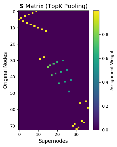
S matrix shape: [73, 37]
Sparse assignment: True
Each node is assigned to exactly one supernode (sparse pooling)

# MinCut pooler (dense assignment)
mincut_vis = get_pooler('mincut', in_channels=2, k=20)

# Apply pooler and get SelectOutput for visualization
pool_out_mincut = mincut_vis(x=pygsp_batch.x, adj=pygsp_batch.edge_index, batch=pygsp_batch.batch)
so_mincut = pool_out_mincut.so

# Visualize S matrix
plt.figure(figsize=(4, 5))
S_matrix = so_mincut.s[0].detach().numpy()  # First graph in batch
plt.imshow(S_matrix, cmap='viridis', aspect='auto')
plt.title(r"$\mathbf{S}$ Matrix (MinCut Pooling) - First Graph", fontsize=14)
plt.xlabel("Supernodes", fontsize=12)
plt.ylabel("Original Nodes", fontsize=12)
plt.colorbar(label='Assignment Weight')
plt.tight_layout()
plt.show()

print(f"S matrix shape: {S_matrix.shape}")
print(f"Soft assignment: {so_mincut.is_expressive}")
print("Nodes can belong to multiple supernodes with different weights (dense pooling)")

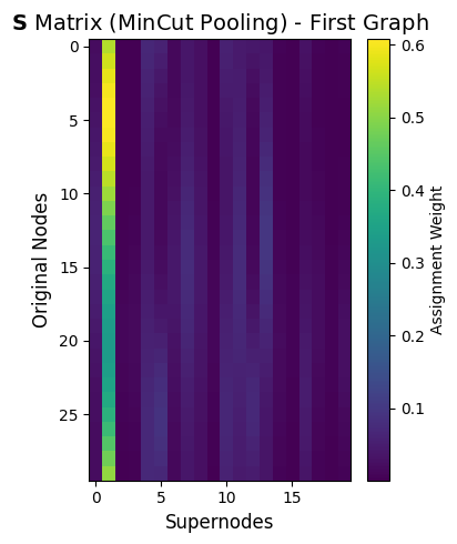
S matrix shape: (30, 20)
Soft assignment: True
Nodes can belong to multiple supernodes with different weights (dense pooling)

Visualizing Graph Coarsening

Now let’s visualize how pooling coarsens the graph structure.

# Visualize original graph
G = to_networkx(pygsp_batch, to_undirected=True)
pos = pygsp_batch.x.numpy()

plt.figure(figsize=(5,5))
nx.draw(G, pos=pos, node_size=20, node_color='lightblue', 
        edge_color='gray', with_labels=False, alpha=0.8)
plt.title("Original Graphs (3 graphs batched)", fontsize=14)
plt.axis('equal')
plt.tight_layout()
plt.show()

print(f"Total nodes: {pygsp_batch.x.shape[0]}")
print(f"Total edges: {pygsp_batch.edge_index.shape[1]}")

/tmp/ipykernel_779/1352153523.py:10: UserWarning: This figure includes Axes that are not compatible with tight_layout, so results might be incorrect.
  plt.tight_layout()

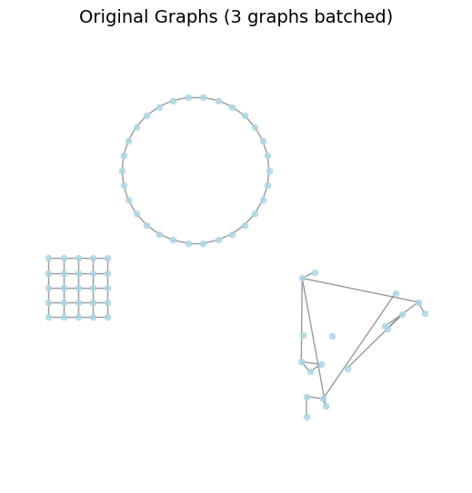
Total nodes: 73
Total edges: 174

# Apply pooling and highlight selected nodes
pool_out = topk_pooler(x=pygsp_batch.x, adj=pygsp_batch.edge_index, batch=pygsp_batch.batch)

# Get indices of selected nodes
selected_indices = pool_out.so.s.indices()[0].numpy()

plt.figure(figsize=(6, 6))
# Draw all nodes in gray
nx.draw(G, pos=pos, node_size=20, node_color='lightgray', 
        edge_color='lightgray', with_labels=False, alpha=0.5)
# Highlight selected nodes in red
nx.draw_networkx_nodes(G, pos=pos, nodelist=selected_indices.tolist(),
                       node_color='red', node_size=20, alpha=0.9)
plt.title(f"After TopK Pooling (red nodes selected, {len(selected_indices)}/{pygsp_batch.x.shape[0]} nodes kept)", 
          fontsize=14)
plt.axis('equal')
plt.tight_layout()
plt.show()

print(f"Selected nodes: {len(selected_indices)} out of {pygsp_batch.x.shape[0]}")
print(f"Reduction ratio: {len(selected_indices)/pygsp_batch.x.shape[0]:.2f}")

/tmp/ipykernel_779/946885220.py:17: UserWarning: This figure includes Axes that are not compatible with tight_layout, so results might be incorrect.
  plt.tight_layout()

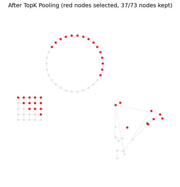
Selected nodes: 37 out of 73
Reduction ratio: 0.51

# Visualize the coarsened graph structure
from torch_geometric.data import Data

# Create Data object for pooled graph
pooled_data = Data(x=pool_out.x, edge_index=pool_out.edge_index, batch=pool_out.batch)
G_pooled = to_networkx(pooled_data, to_undirected=True)

plt.figure(figsize=(5, 5))
# Use pooled features as positions (which are the original positions of selected nodes)
pos_pooled = pool_out.x.detach().numpy()
nx.draw_networkx_nodes(G_pooled, pos=pos_pooled, node_size=20, 
                       node_color=pool_out.batch.numpy(), 
                       cmap='Set3', alpha=0.8)
nx.draw_networkx_edges(G_pooled, pos=pos_pooled, edge_color='gray', 
                       alpha=0.5, width=2)
plt.title("Coarsened Graph Structure", fontsize=14)
plt.axis('equal')
plt.tight_layout()
plt.show()

print(f"Coarsened graph nodes: {pool_out.x.shape[0]}")
print(f"Coarsened graph edges: {pool_out.edge_index.shape[1]}")

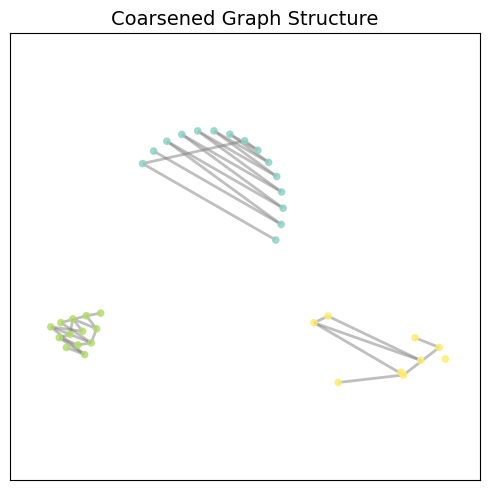
Coarsened graph nodes: 37
Coarsened graph edges: 76

We’ll use the MUTAG dataset for graph classification tasks. This dataset contains 188 chemical compounds (molecules), where each graph represents a molecule and the task is to predict whether it has mutagenic effects on a bacterium (binary classification).

For more information about datasets in PyG, see the PyG documentation.

# Dataset info
print(f'Dataset: {dataset}')
print(f'Number of graphs: {len(dataset)}')
print(f'Number of features: {dataset.num_features}')
print(f'Number of classes: {dataset.num_classes}')

# Create train and test loaders
train_dataset = dataset[:150]
test_dataset = dataset[150:]
train_loader = DataLoader(train_dataset, batch_size=32, shuffle=True)
test_loader = DataLoader(test_dataset, batch_size=32)

# Look at one batch
batch = next(iter(train_loader))
print(f'\nSample batch: {batch}')

Dataset: MUTAG(188)
Number of graphs: 188
Number of features: 7
Number of classes: 2

Sample batch: DataBatch(edge_index=[2, 1246], x=[567, 7], edge_attr=[1246, 4], y=[32], batch=[567], ptr=[33])

Baseline GNN without Pooling

Let’s start by building a simple GNN without graph pooling. This will serve as our baseline to understand the benefits that pooling brings.

Our baseline architecture uses GCNConv layers followed by global sum pooling:

[GCNConv → ReLU → GCNConv → ReLU → GlobalSumPool → Linear]

class BaselineGCN(torch.nn.Module):
    def __init__(self, hidden_channels):
        super(BaselineGCN, self).__init__()
        torch.manual_seed(42)
        
        # Two GCN layers
        self.conv1 = GCNConv(dataset.num_features, hidden_channels)
        self.conv2 = GCNConv(hidden_channels, hidden_channels)
        
        # Readout layer
        self.readout = GlobalReduce(reduce_op="sum")

        # Final classifier
        self.lin = Linear(hidden_channels, dataset.num_classes)

    def forward(self, x, edge_index, batch):
        # 1. Obtain node embeddings through GCN layers
        x = self.conv1(x, edge_index)
        x = x.relu()
        x = self.conv2(x, edge_index)
        x = x.relu()

        # 2. Readout layer: aggregate node features to graph-level
        x = self.readout(x, batch=batch)  # [batch_size, hidden_channels]

        # 3. Apply final classifier
        x = F.dropout(x, p=0.5, training=self.training)
        x = self.lin(x)
        
        return x

baseline_model = BaselineGCN(hidden_channels=64)
print(baseline_model)

BaselineGCN(
  (conv1): GCNConv(7, 64)
  (conv2): GCNConv(64, 64)
  (readout): GlobalReduce(aggr=SumAggregation())
  (lin): Linear(in_features=64, out_features=2, bias=True)
)

Readout: global pooling with tgp

Here we perform global sum pooling using tgp’s readout: GlobalReduce(reduce_op="sum"). It aggregates node features to one vector per graph (sum over nodes in each graph, using batch to group).

The readout uses aggregators—the same concept as PyTorch Geometric’s aggregation operators. You can pass a string alias (e.g. "sum", "mean", "max") to reduce_op, or any PyG Aggregation instance; tgp resolves strings via get_aggr and uses them to combine features. So when you see (readout): GlobalReduce(aggr=SumAggregation()) in the model printout, that is the sum aggregator in use.

For other aggregations and for AggrReduce (e.g. when reducing with a custom PyG module), see the Advanced tutorial.

Let’s train the baseline model:

device = torch.device('cuda' if torch.cuda.is_available() else 'cpu')
model = baseline_model.to(device)
optimizer = torch.optim.Adam(model.parameters(), lr=0.01)
criterion = torch.nn.CrossEntropyLoss()

def train():
    model.train()
    total_loss = 0
    for data in train_loader:
        data = data.to(device)
        optimizer.zero_grad()
        out = model(data.x, data.edge_index, data.batch)
        loss = criterion(out, data.y)
        loss.backward()
        optimizer.step()
        total_loss += loss.item() * data.num_graphs
    return total_loss / len(train_loader.dataset)

@torch.no_grad()
def test(loader):
    model.eval()
    correct = 0
    for data in loader:
        data = data.to(device)
        out = model(data.x, data.edge_index, data.batch)
        pred = out.argmax(dim=1)
        correct += int((pred == data.y).sum())
    return correct / len(loader.dataset)

print("Training baseline GNN (no pooling)...")
for epoch in range(1, 51):
    loss = train()
    train_acc = test(train_loader)
    test_acc = test(test_loader)
    if epoch % 5 == 0:
        print(f'Epoch: {epoch:03d}, Loss: {loss:.4f}, Train Acc: {train_acc:.4f}, Test Acc: {test_acc:.4f}')

print(f'\nFinal Test Accuracy (Baseline): {test_acc:.4f}')

Training baseline GNN (no pooling)...

Epoch: 005, Loss: 0.5687, Train Acc: 0.6600, Test Acc: 0.7105
Epoch: 010, Loss: 0.4977, Train Acc: 0.7533, Test Acc: 0.6842

Epoch: 015, Loss: 0.4780, Train Acc: 0.7533, Test Acc: 0.7105
Epoch: 020, Loss: 0.4614, Train Acc: 0.7867, Test Acc: 0.7105

Epoch: 025, Loss: 0.4470, Train Acc: 0.7867, Test Acc: 0.6842

Epoch: 030, Loss: 0.4766, Train Acc: 0.7933, Test Acc: 0.6842

Epoch: 035, Loss: 0.4782, Train Acc: 0.7933, Test Acc: 0.7632

Epoch: 040, Loss: 0.4560, Train Acc: 0.7933, Test Acc: 0.6842
Epoch: 045, Loss: 0.4399, Train Acc: 0.7867, Test Acc: 0.7105

Epoch: 050, Loss: 0.4657, Train Acc: 0.8000, Test Acc: 0.7632

Final Test Accuracy (Baseline): 0.7632

Adding Pooling to a GNN

Now let’s see how easy it is to add graph pooling to our GNN! We simply insert a pooling layer between message-passing layers.

Our new architecture with MaxCutPooling:

[GCNConv → MaxCutPool → GCNConv → GlobalSumPool → Linear]

Notice how easy it is - we just add one line with get_pooler()!

class GNNWithPooling(torch.nn.Module):
    def __init__(self, hidden_channels=64):
        super().__init__()
        
        # First GCN layer
        self.conv1 = GCNConv(dataset.num_features, hidden_channels)
        
        # Pooling layer - easily added with get_pooler!
        self.pooler = get_pooler('maxcut', in_channels=hidden_channels, ratio=0.5)
        
        # Second GCN layer (after pooling)
        self.conv2 = GCNConv(hidden_channels, hidden_channels)
        
        # Readout layer
        self.readout = GlobalReduce(reduce_op="sum")

        # Classifier
        self.lin = Linear(hidden_channels, dataset.num_classes)
    
    def forward(self, x, edge_index, edge_weight, batch):
        # First GCN layer
        x = self.conv1(x, edge_index, edge_weight)
        x = F.relu(x)
        
        # Pooling: coarsen the graph
        pool_out = self.pooler(x=x, adj=edge_index, edge_weight=edge_weight, batch=batch)
        x_pooled = pool_out.x
        edge_index_pooled = pool_out.edge_index
        edge_weight_pooled = pool_out.edge_weight
        batch_pooled = pool_out.batch
        
        # Second GCN layer on the pooled graph
        x = self.conv2(x_pooled, edge_index_pooled, edge_weight_pooled)
        x = F.relu(x)
        
        # Global pooling
        x = self.readout(x, batch=batch_pooled)
        
        # Classifier
        x = F.dropout(x, p=0.5, training=self.training)
        x = self.lin(x)
        
        return x

pooling_model = GNNWithPooling(hidden_channels=64)
print(pooling_model)
print(f"\nPooler details:")
print(pooling_model.pooler)

GNNWithPooling(
  (conv1): GCNConv(7, 64)
  (pooler): MaxCutPooling(
  	select=MaxCutSelect(in_channels=64, ratio=0.5, assign_all_nodes=True, mp_units=[32, 32, 32, 32], mp_act='tanh', mlp_units=[16, 16], mlp_act='relu', act='tanh', delta=2.0, max_iter=5)
  	reduce=BaseReduce()
  	lift=BaseLift(matrix_op=precomputed, reduce_op=sum)
  	connect=SparseConnect(reduce_op=sum, remove_self_loops=True, edge_weight_norm=True, degree_norm=False)
  	loss_coeff=1.0
  )
  (conv2): GCNConv(64, 64)
  (readout): GlobalReduce(aggr=SumAggregation())
  (lin): Linear(in_features=64, out_features=2, bias=True)
)

Pooler details:
MaxCutPooling(
	select=MaxCutSelect(in_channels=64, ratio=0.5, assign_all_nodes=True, mp_units=[32, 32, 32, 32], mp_act='tanh', mlp_units=[16, 16], mlp_act='relu', act='tanh', delta=2.0, max_iter=5)
	reduce=BaseReduce()
	lift=BaseLift(matrix_op=precomputed, reduce_op=sum)
	connect=SparseConnect(reduce_op=sum, remove_self_loops=True, edge_weight_norm=True, degree_norm=False)
	loss_coeff=1.0
)

Notice how the pooler shows its internal SRC components: select, reduce, lift, and connect.

Let’s train this model:

model = pooling_model.to(device)
optimizer = torch.optim.Adam(model.parameters(), lr=0.01)

def train():
    model.train()
    total_loss = 0
    for data in train_loader:
        data = data.to(device)
        optimizer.zero_grad()
        out = model(data.x, data.edge_index, data.edge_weight, data.batch)
        loss = criterion(out, data.y)
        loss.backward()
        optimizer.step()
        total_loss += loss.item() * data.num_graphs
    return total_loss / len(train_loader.dataset)

@torch.no_grad()
def test(loader):
    model.eval()
    correct = 0
    for data in loader:
        data = data.to(device)
        out = model(data.x, data.edge_index, data.edge_weight, data.batch)
        pred = out.argmax(dim=1)
        correct += int((pred == data.y).sum())
    return correct / len(loader.dataset)

print("Training GNN with pooling...")
for epoch in range(1, 51):
    loss = train()
    train_acc = test(train_loader)
    test_acc = test(test_loader)
    if epoch % 5 == 0:
        print(f'Epoch: {epoch:03d}, Loss: {loss:.4f}, Train Acc: {train_acc:.4f}, Test Acc: {test_acc:.4f}')

print(f'\nFinal Test Accuracy (with pooling): {test_acc:.4f}')

Training GNN with pooling...

Epoch: 005, Loss: 0.5866, Train Acc: 0.6600, Test Acc: 0.6842

Epoch: 010, Loss: 0.5074, Train Acc: 0.7400, Test Acc: 0.6842

Epoch: 015, Loss: 0.4309, Train Acc: 0.7533, Test Acc: 0.7105

Epoch: 020, Loss: 0.4838, Train Acc: 0.7933, Test Acc: 0.7105

Epoch: 025, Loss: 0.4695, Train Acc: 0.7933, Test Acc: 0.6579

Epoch: 030, Loss: 0.4449, Train Acc: 0.8200, Test Acc: 0.6842

Epoch: 035, Loss: 0.4208, Train Acc: 0.8200, Test Acc: 0.7632

Epoch: 040, Loss: 0.4258, Train Acc: 0.8400, Test Acc: 0.7895

Epoch: 045, Loss: 0.3752, Train Acc: 0.8600, Test Acc: 0.7632

Epoch: 050, Loss: 0.4043, Train Acc: 0.8667, Test Acc: 0.6842

Final Test Accuracy (with pooling): 0.6842

Dense Poolers and Auxiliary Losses

tgp supports two types of pooling operators:

• Sparse poolers: Work with edge lists (like TopK, SAG, ASAP)

• Dense poolers: In their default configuration, work with dense adjacency matrices (like MinCut, DiffPool, DMoN)

Dense poolers often come with auxiliary losses that help guide the learning process (e.g., the cut loss and orthogonality loss in MinCutPooling).

Let’s explore MinCut pooling:

# Create a MinCut pooler (dense)
dense_pooler = get_pooler('mincut', in_channels=7, k=20)
print("MinCut pooler (dense):")
print(dense_pooler)
print(f"\nIs dense? {dense_pooler.is_dense}")
print(f"Has auxiliary loss? Check the cut_loss_coeff and ortho_loss_coeff parameters")

MinCut pooler (dense):
MinCutPooling(
	select=MLPSelect(in_channels=[7], k=20, act=None, dropout=0.0, s_inv_op=transpose)
	reduce=BaseReduce()
	lift=BaseLift(matrix_op=precomputed, reduce_op=sum)
	connect=DenseConnect(remove_self_loops=True, degree_norm=True, adj_transpose=True, edge_weight_norm=False, sparse_output=False)
	batched=True
	cut_loss_coeff=1.0
	ortho_loss_coeff=1.0
)

Is dense? True
Has auxiliary loss? Check the cut_loss_coeff and ortho_loss_coeff parameters

Let’s apply the dense pooler and examine the auxiliary losses:

# Apply dense pooling
dense_pool_out = dense_pooler(x=batch.x, adj=batch.edge_index, batch=batch.batch)

print("Dense pooling output:")
print(dense_pool_out)
print(f"\nPooled graph has {dense_pool_out.so.num_supernodes} supernodes (as specified)")
print(f"\nAuxiliary losses:")
for loss_name, loss_value in dense_pool_out.loss.items():
    print(f"  {loss_name}: {loss_value:.4f}")

Dense pooling output:
PoolingOutput(so=[28, 20], x=[32, 20, 7], edge_index=[32, 20, 20], edge_weight=None, batch=None, mask=[32, 20], loss=['cut_loss', 'ortho_loss'])

Pooled graph has 20 supernodes (as specified)

Auxiliary losses:
  cut_loss: -0.9865
  ortho_loss: 1.2429

Building a GNN with Dense Pooling

When using dense poolers in their default configuration, we need to:

1. Use DenseGCNConv layers after pooling (instead of regular GCNConv)

2. Add auxiliary losses to the total loss during training

class GNNWithDensePooling(torch.nn.Module):
    def __init__(self, hidden_channels=64):
        super().__init__()
        
        # First GCN layer (sparse)
        self.conv1 = GCNConv(dataset.num_features, hidden_channels)
        
        # Dense pooling layer
        self.pooler = get_pooler('mincut', in_channels=hidden_channels, k=20, cut_loss_coeff=0.01, ortho_loss_coeff=0.01)
        
        # Second GCN layer (dense, because pooler is dense)
        self.conv2 = DenseGCNConv(hidden_channels, hidden_channels)
        
        # Readout layer
        self.readout = GlobalReduce(reduce_op="sum")

        # Classifier
        self.lin = Linear(hidden_channels, dataset.num_classes)
    
    def forward(self, x, edge_index, edge_weight, batch):
        # First GCN layer
        x = self.conv1(x, edge_index, edge_weight)
        x = F.relu(x)
        
        # Dense pooling
        pool_out = self.pooler(x=x, adj=edge_index, edge_weight=edge_weight, batch=batch)
        
        # Second GCN layer (on dense adjacency)
        x = self.conv2(pool_out.x, pool_out.edge_index)
        x = F.relu(x)
        
        # Global pooling
        x = self.readout(x, batch=None)  # batch=None for dense
        
        # Classifier
        x = F.dropout(x, p=0.5, training=self.training)
        x = self.lin(x)
        
        # Return predictions and auxiliary loss
        aux_loss = sum(pool_out.get_loss_value()) if pool_out.loss else 0.0
        return x, aux_loss

dense_model = GNNWithDensePooling(hidden_channels=64)
print(dense_model)

GNNWithDensePooling(
  (conv1): GCNConv(7, 64)
  (pooler): MinCutPooling(
  	select=MLPSelect(in_channels=[64], k=20, act=None, dropout=0.0, s_inv_op=transpose)
  	reduce=BaseReduce()
  	lift=BaseLift(matrix_op=precomputed, reduce_op=sum)
  	connect=DenseConnect(remove_self_loops=True, degree_norm=True, adj_transpose=True, edge_weight_norm=False, sparse_output=False)
  	batched=True
  	cut_loss_coeff=0.01
  	ortho_loss_coeff=0.01
  )
  (conv2): DenseGCNConv(64, 64)
  (readout): GlobalReduce(aggr=SumAggregation())
  (lin): Linear(in_features=64, out_features=2, bias=True)
)

Training with auxiliary losses - note how we add aux_loss to the total loss:

model = dense_model.to(device)
optimizer = torch.optim.Adam(model.parameters(), lr=0.01)

def train_with_aux_loss():
    model.train()
    total_loss = 0
    for data in train_loader:
        data = data.to(device)
        optimizer.zero_grad()
        out, aux_loss = model(data.x, data.edge_index, data.edge_weight, data.batch)
        loss = criterion(out, data.y) + aux_loss  # Add auxiliary loss!
        loss.backward()
        optimizer.step()
        total_loss += loss.item() * data.num_graphs
    return total_loss / len(train_loader.dataset)

@torch.no_grad()
def test_with_aux(loader):
    model.eval()
    correct = 0
    for data in loader:
        data = data.to(device)
        out, _ = model(data.x, data.edge_index, data.edge_weight, data.batch)
        pred = out.argmax(dim=1)
        correct += int((pred == data.y).sum())
    return correct / len(loader.dataset)

print("Training GNN with dense pooling and auxiliary losses...")
for epoch in range(1, 51):
    loss = train_with_aux_loss()
    train_acc = test_with_aux(train_loader)
    test_acc = test_with_aux(test_loader)
    if epoch % 5 == 0:
        print(f'Epoch: {epoch:03d}, Loss: {loss:.4f}, Train Acc: {train_acc:.4f}, Test Acc: {test_acc:.4f}')

print(f'\nFinal Test Accuracy (Dense Pooling): {test_acc:.4f}')

Training GNN with dense pooling and auxiliary losses...

Epoch: 005, Loss: 0.4888, Train Acc: 0.8533, Test Acc: 0.8158

Epoch: 010, Loss: 0.3965, Train Acc: 0.8533, Test Acc: 0.7895

Epoch: 015, Loss: 0.3630, Train Acc: 0.8533, Test Acc: 0.8158

Epoch: 020, Loss: 0.3792, Train Acc: 0.8533, Test Acc: 0.7895

Epoch: 025, Loss: 0.3786, Train Acc: 0.8600, Test Acc: 0.8158

Epoch: 030, Loss: 0.3372, Train Acc: 0.8667, Test Acc: 0.7895

Epoch: 035, Loss: 0.4222, Train Acc: 0.8333, Test Acc: 0.7895

Epoch: 040, Loss: 0.4212, Train Acc: 0.8600, Test Acc: 0.7368

Epoch: 045, Loss: 0.3195, Train Acc: 0.8533, Test Acc: 0.7632

Epoch: 050, Loss: 0.3241, Train Acc: 0.8600, Test Acc: 0.7895

Final Test Accuracy (Dense Pooling): 0.7895

Dense Poolers: Input/Output Flexibility

Dense poolers in tgp are highly flexible. They support different configurations via the batched and sparse_output flags:

Configuration	batched	sparse_output	Input	Internal Representation	Output
Batched Dense	True (default)	False (default)	Sparse edge list/Dense adjacency	Dense (padded tensors)	Dense adjacency
Batched Sparse	True	True	Sparse edge list/Dense adjacency	Dense (padded tensors)	Sparse edge list
Unbatched Dense	False	False	Sparse edge list	Sparse (per-graph loops)	Dense adjacency
Unbatched Sparse	False	True	Sparse edge list	Sparse (per-graph loops)	Sparse edge list

The internal representation determines the pooling operations: dense operations are vectorized and faster but use more memory due to padding, while sparse operations are memory-efficient but slower due to per-graph processing. This allows you to trade off between time and space based on your specific needs.

For details on when to use each mode and the trade-offs involved, see the tgp paper.

# Create 4 MinCut configurations
configs = [
    ('Batched Dense', dict(batched=True, sparse_output=False)),
    ('Batched Sparse', dict(batched=True, sparse_output=True)),
    ('Unbatched Dense', dict(batched=False, sparse_output=False)),
    ('Unbatched Sparse', dict(batched=False, sparse_output=True)),
]

batch = next(iter(train_loader))

print(f"Batch: {batch}")

for name, config in configs:
    pooler = get_pooler('mincut', in_channels=7, k=10, **config)
    out = pooler(x=batch.x, adj=batch.edge_index, batch=batch.batch)
    
    # Get output shapes
    x_shape = out.x.shape
    adj_shape = out.edge_index.shape if out.edge_index.dim() == 2 else f"{out.edge_index.shape} (dense)"
    
    print(f"\n{name}:")
    print(f"  pooler.batched = {pooler.batched}")
    print(f"  pooler.sparse_output = {pooler.sparse_output}")
    print(f"  Output x shape: {x_shape}")
    print(f"  Output edge_index shape: {adj_shape}")

Batch: DataBatch(edge_index=[2, 1244], x=[561, 7], edge_attr=[1244, 4], y=[32], batch=[561], ptr=[33])

Batched Dense:
  pooler.batched = True
  pooler.sparse_output = False
  Output x shape: torch.Size([32, 10, 7])
  Output edge_index shape: torch.Size([32, 10, 10]) (dense)

Batched Sparse:
  pooler.batched = True
  pooler.sparse_output = True
  Output x shape: torch.Size([320, 7])
  Output edge_index shape: torch.Size([2, 2880])

Unbatched Dense:
  pooler.batched = False
  pooler.sparse_output = False
  Output x shape: torch.Size([32, 10, 7])
  Output edge_index shape: torch.Size([32, 10, 10]) (dense)

Unbatched Sparse:
  pooler.batched = False
  pooler.sparse_output = True
  Output x shape: torch.Size([320, 7])
  Output edge_index shape: torch.Size([2, 2880])

Trade-offs:

• Batched mode (batched=True): Efficient for batches of small graphs, but requires padding to handle variable-sized graphs

• Unbatched mode (batched=False): Processes graphs one at a time, avoiding padding overhead for large graphs

• Dense output (sparse_output=False): Required if using dense layers (like DenseGCNConv) after pooling

• Sparse output (sparse_output=True): Allows using regular sparse layers after pooling, reducing memory for large graphs

Hierarchical Architectures

One of the key benefits of graph pooling is building truly hierarchical architectures with multiple pooling layers. This allows the network to learn features at different scales.

Architecture with 2 pooling layers:

[GCN → Pool₁ → GCN → Pool₂ → GCN → GlobalSumPool → Linear]

class HierarchicalGNN(torch.nn.Module):
    def __init__(self, hidden_channels=64):
        super().__init__()
        
        # First GCN layer
        self.conv1 = GCNConv(dataset.num_features, hidden_channels)
        
        # First pooling layer (keep 50% of nodes)
        self.pooler1 = get_pooler('topk', in_channels=hidden_channels, ratio=0.5)
        
        # Second GCN layer
        self.conv2 = GCNConv(hidden_channels, hidden_channels)
        
        # Second pooling layer (keep 50% of remaining nodes)
        self.pooler2 = get_pooler('topk', in_channels=hidden_channels, ratio=0.5)
        
        # Third GCN layer
        self.conv3 = GCNConv(hidden_channels, hidden_channels)

        # Readout layer
        self.readout = GlobalReduce(reduce_op="sum")
        
        # Classifier
        self.lin = Linear(hidden_channels, dataset.num_classes)
    
    def forward(self, x, edge_index, edge_weight, batch):
        # First GCN layer
        x = self.conv1(x, edge_index, edge_weight)
        x = F.relu(x)
        
        # First pooling
        out1 = self.pooler1(x=x, adj=edge_index, edge_weight=edge_weight, batch=batch)
        
        # Second GCN layer
        x = self.conv2(out1.x, out1.edge_index, out1.edge_weight)
        x = F.relu(x)
        
        # Second pooling
        out2 = self.pooler2(x=x, adj=out1.edge_index, edge_weight=out1.edge_weight, batch=out1.batch)
        
        # Third GCN layer
        x = self.conv3(out2.x, out2.edge_index, out2.edge_weight)
        x = F.relu(x)
        
        # Global pooling
        x = self.readout(x, batch=out2.batch)
        
        # Classifier
        x = F.dropout(x, p=0.5, training=self.training)
        x = self.lin(x)
        
        # Combine auxiliary losses from both poolers (if any)
        total_aux_loss = 0.0
        if out1.loss:
            total_aux_loss += sum(out1.get_loss_value())
        if out2.loss:
            total_aux_loss += sum(out2.get_loss_value())
        
        return x, total_aux_loss

hierarchical_model = HierarchicalGNN(hidden_channels=64)
print(hierarchical_model)

HierarchicalGNN(
  (conv1): GCNConv(7, 64)
  (pooler1): TopkPooling(
  	select=TopkSelect(in_channels=64, ratio=0.5, act=Tanh(), s_inv_op=transpose)
  	reduce=BaseReduce()
  	lift=BaseLift(matrix_op=precomputed, reduce_op=sum)
  	connect=SparseConnect(reduce_op=sum, remove_self_loops=True, edge_weight_norm=False, degree_norm=False)
  	multiplier=1.0
  )
  (conv2): GCNConv(64, 64)
  (pooler2): TopkPooling(
  	select=TopkSelect(in_channels=64, ratio=0.5, act=Tanh(), s_inv_op=transpose)
  	reduce=BaseReduce()
  	lift=BaseLift(matrix_op=precomputed, reduce_op=sum)
  	connect=SparseConnect(reduce_op=sum, remove_self_loops=True, edge_weight_norm=False, degree_norm=False)
  	multiplier=1.0
  )
  (conv3): GCNConv(64, 64)
  (readout): GlobalReduce(aggr=SumAggregation())
  (lin): Linear(in_features=64, out_features=2, bias=True)
)

Let’s train the hierarchical model:

model = hierarchical_model.to(device)
optimizer = torch.optim.Adam(model.parameters(), lr=0.01)

print("Training hierarchical GNN (2 pooling layers)...")
for epoch in range(1, 51):
    loss = train_with_aux_loss()
    train_acc = test_with_aux(train_loader)
    test_acc = test_with_aux(test_loader)
    if epoch % 5 == 0:
        print(f'Epoch: {epoch:03d}, Loss: {loss:.4f}, Train Acc: {train_acc:.4f}, Test Acc: {test_acc:.4f}')

print(f'\nFinal Test Accuracy (Hierarchical with 2 pooling layers): {test_acc:.4f}')

Training hierarchical GNN (2 pooling layers)...

Epoch: 005, Loss: 0.5773, Train Acc: 0.6600, Test Acc: 0.6842

Epoch: 010, Loss: 0.5860, Train Acc: 0.7800, Test Acc: 0.7368

Epoch: 015, Loss: 0.5101, Train Acc: 0.7600, Test Acc: 0.7368

Epoch: 020, Loss: 0.4941, Train Acc: 0.7800, Test Acc: 0.7632

Epoch: 025, Loss: 0.5423, Train Acc: 0.7867, Test Acc: 0.7368

Epoch: 030, Loss: 0.5079, Train Acc: 0.7733, Test Acc: 0.7368

Epoch: 035, Loss: 0.4851, Train Acc: 0.7867, Test Acc: 0.7368

Epoch: 040, Loss: 0.4938, Train Acc: 0.7733, Test Acc: 0.7368

Epoch: 045, Loss: 0.4794, Train Acc: 0.7733, Test Acc: 0.7368

Epoch: 050, Loss: 0.4924, Train Acc: 0.7733, Test Acc: 0.7368

Final Test Accuracy (Hierarchical with 2 pooling layers): 0.7368

Caching for Single-Graph Tasks

For tasks involving a single large graph (like node classification), the pooler is called with ((x, adj)) and the decoder can use the original graph’s adjacency.

Let’s switch to the Cora dataset, a citation network where we classify research papers into topics:

# Load Cora dataset
cora_dataset = Planetoid(root='/tmp/Cora', name='Cora')
cora_data = cora_dataset[0]

print(f'Dataset: {cora_dataset}')
print(f'Data: {cora_data}')
print(f'Number of nodes: {cora_data.num_nodes}')
print(f'Number of edges: {cora_data.num_edges}')
print(f'Number of features: {cora_dataset.num_features}')
print(f'Number of classes: {cora_dataset.num_classes}')

Downloading https://github.com/kimiyoung/planetoid/raw/master/data/ind.cora.x

Downloading https://github.com/kimiyoung/planetoid/raw/master/data/ind.cora.tx

Downloading https://github.com/kimiyoung/planetoid/raw/master/data/ind.cora.allx

Downloading https://github.com/kimiyoung/planetoid/raw/master/data/ind.cora.y
Downloading https://github.com/kimiyoung/planetoid/raw/master/data/ind.cora.ty

Downloading https://github.com/kimiyoung/planetoid/raw/master/data/ind.cora.ally

Downloading https://github.com/kimiyoung/planetoid/raw/master/data/ind.cora.graph

Dataset: Cora()
Data: Data(x=[2708, 1433], edge_index=[2, 10556], y=[2708], train_mask=[2708], val_mask=[2708], test_mask=[2708])
Number of nodes: 2708
Number of edges: 10556
Number of features: 1433
Number of classes: 7

Downloading https://github.com/kimiyoung/planetoid/raw/master/data/ind.cora.test.index
Processing...
Done!

For node classification, we often use an encoder-decoder architecture with pooling and \(\texttt{LIFT}\) in the middle:

[Encoder → Pool → Bottleneck → LIFT → Decoder]

The pooler is called with ((x, adj, batch)) directly; for the decoder we use the original graph’s adjacency (e.g. via to_dense_adj).

class NodeClassificationGNN(torch.nn.Module):
    def __init__(self, hidden_channels=16):
        super().__init__()
        
        # Encoder
        self.conv_enc = GCNConv(cora_dataset.num_features, hidden_channels)
        
        # Pooler
        self.pooler = get_pooler(
            'mincut',
            in_channels=hidden_channels,
            k=cora_data.num_nodes // 20,  # Coarsen to ~5% of original size
            sparse_output=False
        )
        
        # Bottleneck (on pooled graph)
        self.conv_pool = DenseGCNConv(hidden_channels, hidden_channels // 2)
        
        # Decoder (after lifting)
        self.conv_dec = DenseGCNConv(hidden_channels // 2, cora_dataset.num_classes)
    
    def forward(self, x, edge_index, edge_weight):
        # Encoder
        x = self.conv_enc(x, edge_index, edge_weight)
        x = F.relu(x)
        x = F.dropout(x, p=0.5, training=self.training)
        
        # Pool
        pool_out = self.pooler(x=x, adj=edge_index, edge_weight=edge_weight, batch=None)
        
        # Bottleneck
        x_pool = self.conv_pool(pool_out.x, pool_out.edge_index)
        x_pool = F.relu(x_pool)
        x_pool = F.dropout(x_pool, p=0.5, training=self.training)
        
        # Lift back to original space
        x_lift = self.pooler(x=x_pool, so=pool_out.so, lifting=True, batch=None)
        
        # Decoder (dense adj for single graph)
        adj_dense = to_dense_adj(edge_index)
        x = self.conv_dec(x_lift, adj_dense)
        
        # Extract from batch dimension
        if x.dim() == 3:
            x = x[0]
        
        # Return predictions and auxiliary loss
        aux_loss = sum(pool_out.get_loss_value()) if pool_out.loss else 0.0
        return F.log_softmax(x, dim=-1), aux_loss

node_model = NodeClassificationGNN(hidden_channels=16)
print(node_model)

NodeClassificationGNN(
  (conv_enc): GCNConv(1433, 16)
  (pooler): MinCutPooling(
  	select=MLPSelect(in_channels=[16], k=135, act=None, dropout=0.0, s_inv_op=transpose)
  	reduce=BaseReduce()
  	lift=BaseLift(matrix_op=precomputed, reduce_op=sum)
  	connect=DenseConnect(remove_self_loops=True, degree_norm=True, adj_transpose=True, edge_weight_norm=False, sparse_output=False)
  	batched=True
  	cut_loss_coeff=1.0
  	ortho_loss_coeff=1.0
  )
  (conv_pool): DenseGCNConv(16, 8)
  (conv_dec): DenseGCNConv(8, 7)
)

Training for node classification (we only train on labeled nodes):

model = node_model.to(device)
cora_data = cora_data.to(device)
optimizer = torch.optim.Adam(model.parameters(), lr=0.01, weight_decay=5e-4)

def train_node():
    model.train()
    optimizer.zero_grad()
    out, aux_loss = model(cora_data.x, cora_data.edge_index, cora_data.edge_weight)
    loss = F.nll_loss(out[cora_data.train_mask], cora_data.y[cora_data.train_mask]) + aux_loss
    loss.backward()
    optimizer.step()
    return loss.item()

@torch.no_grad()
def test_node():
    model.eval()
    out, _ = model(cora_data.x, cora_data.edge_index, cora_data.edge_weight)
    pred = out.argmax(dim=1)
    
    accs = []
    for mask in [cora_data.train_mask, cora_data.val_mask, cora_data.test_mask]:
        correct = pred[mask].eq(cora_data.y[mask]).sum().item()
        acc = correct / mask.sum().item()
        accs.append(acc)
    return accs

print("Training node classification with caching...")
for epoch in range(1, 201):
    loss = train_node()
    train_acc, val_acc, test_acc = test_node()
    if epoch % 20 == 0:
        print(f'Epoch: {epoch:03d}, Loss: {loss:.4f}, Train: {train_acc:.4f}, Val: {val_acc:.4f}, Test: {test_acc:.4f}')

print(f'\nFinal Test Accuracy: {test_acc:.4f}')

Training node classification with caching...

Epoch: 020, Loss: 2.2989, Train: 0.1571, Val: 0.1200, Test: 0.1030

Epoch: 040, Loss: 2.2945, Train: 0.1429, Val: 0.1220, Test: 0.1300

Epoch: 060, Loss: 2.2884, Train: 0.1500, Val: 0.1260, Test: 0.1270

Epoch: 080, Loss: 2.2827, Train: 0.1429, Val: 0.1420, Test: 0.1200

Epoch: 100, Loss: 2.2787, Train: 0.1714, Val: 0.1760, Test: 0.1430

Epoch: 120, Loss: 2.2752, Train: 0.1571, Val: 0.1840, Test: 0.1440

Epoch: 140, Loss: 2.2728, Train: 0.1714, Val: 0.1760, Test: 0.1460

Epoch: 160, Loss: 2.2718, Train: 0.1714, Val: 0.1580, Test: 0.1480

Epoch: 180, Loss: 2.2726, Train: 0.1786, Val: 0.1580, Test: 0.1380

Epoch: 200, Loss: 2.2716, Train: 0.1714, Val: 0.1540, Test: 0.1330

Final Test Accuracy: 0.1330

Precoarsening for Non-Learnable Poolers

Some pooling operators are non-learnable - they compute node assignments based solely on the graph structure, not on learned node features. Examples include:

• NDPPooling (Node Decimation Pooling)

• GraclusPooling

• NMFPooling

Since the graph structure doesn’t change during training, we can precompute the pooling operations using PreCoarsening!

For advanced precoarsening usages (multiple poolers, different configs per level), see the Precoarsening and transforms notebook.

# Create a non-learnable pooler
ndp_pooler = get_pooler('ndp')  # Node Decimation Pooling
print(f"NDP Pooler: {ndp_pooler}")

# Apply PreCoarsening transform to the dataset
# This will precompute pooling for 2 levels
precoarsened_dataset = TUDataset(
    root='/tmp/MUTAG_precoarsened',
    name='MUTAG',
    pre_transform=PreCoarsening(
        poolers=[ndp_pooler, ndp_pooler]
    ),
    force_reload=True
)

print(f"\nDataset with precoarsening:")
sample = precoarsened_dataset[0]
print(sample)
print(f"\nPooled data levels: {len(sample.pooled_data)}")
for i, pooled in enumerate(sample.pooled_data):
    print(f"  Level {i+1}: {pooled}")

NDP Pooler: NDPPooling(
	select=NDPSelect(s_inv_op=transpose)
	reduce=BaseReduce()
	lift=BaseLift(matrix_op=precomputed, reduce_op=sum)
	connect=KronConnect(sparse_threshold=0.01)
	cached=False
)

Downloading https://www.chrsmrrs.com/graphkerneldatasets/MUTAG.zip

Processing...

Done!
/home/docs/checkouts/readthedocs.org/user_builds/torch-geometric-pool/envs/latest/lib/python3.10/site-packages/torch_geometric/datasets/tu_dataset.py:132: UserWarning: Weights only load failed. Please file an issue to make `torch.load(weights_only=True)` compatible in your case. Please use `torch.serialization.add_safe_globals([torch_geometric.data.data.DataEdgeAttr])` to allowlist this global.
  out = fs.torch_load(self.processed_paths[0])

Dataset with precoarsening:
Data(edge_index=[2, 38], x=[17, 7], edge_attr=[38, 4], y=[1], pooled_data=[2])

Pooled data levels: 2
  Level 1: Data(edge_index=[2, 28], edge_weight=[28], batch=[9], so=SelectOutput(num_nodes=17, num_supernodes=9, extra={'L'}), num_nodes=9)
  Level 2: Data(edge_index=[2, 16], edge_weight=[16], batch=[5], so=SelectOutput(num_nodes=9, num_supernodes=5, extra={'L'}), num_nodes=5)

We need a special PoolDataLoader to properly batch graphs with precoarsened data:

# Use PoolDataLoader instead of regular DataLoader
precoarsened_train = precoarsened_dataset[:150]
precoarsened_test = precoarsened_dataset[150:]

pool_train_loader = PoolDataLoader(precoarsened_train, batch_size=32, shuffle=True)
pool_test_loader = PoolDataLoader(precoarsened_test, batch_size=32)

# Check a batch
batch = next(iter(pool_train_loader))
print(f"Batch: {batch}")
print(f"\nPooled data (properly batched):")
for i, pooled in enumerate(batch.pooled_data):
    print(f"  Level {i+1}: {pooled}")

Batch: DataPooledBatch(edge_index=[2, 1270], x=[578, 7], edge_attr=[1270, 4], y=[32], pooled_data=[2], batch=[578], ptr=[33])

Pooled data (properly batched):
  Level 1: Data(edge_index=[2, 922], edge_weight=[922], batch=[291], so=SelectOutput(num_nodes=578, num_supernodes=291, extra={'L'}), num_nodes=291, ptr=[33])
  Level 2: Data(edge_index=[2, 528], edge_weight=[528], batch=[155], so=SelectOutput(num_nodes=291, num_supernodes=155, extra={'L'}), num_nodes=155, ptr=[33])

Now we can build a model that uses the precomputed pooling structure. Notice that we only need BaseReduce - the \(\texttt{SEL}\) and \(\texttt{CON}\) operations are already precomputed!

class PrecoarsenedGNN(torch.nn.Module):
    def __init__(self, hidden_channels=64):
        super().__init__()
        
        num_features = precoarsened_dataset.num_features
        num_classes = precoarsened_dataset.num_classes
        
        # First MP layer
        self.conv1 = ARMAConv(num_features, hidden_channels, num_layers=2)
        
        # Reducer (we only need REDUCE, SEL and CON are precomputed!)
        self.reducer = BaseReduce()
        
        # MP layers after each pooling level
        self.conv2 = ARMAConv(hidden_channels, hidden_channels, num_layers=2)
        self.conv3 = ARMAConv(hidden_channels, hidden_channels, num_layers=2)
        
        # Readout layer
        self.readout = GlobalReduce(reduce_op="sum")

        # Classifier
        self.lin = Linear(hidden_channels, num_classes)
    
    def forward(self, data):
        # First MP layer on original graph
        x = self.conv1(data.x, data.edge_index, data.edge_weight)
        x = F.relu(x)
        
        # Apply precoarsened pooling levels
        # Level 1
        pooled_1 = data.pooled_data[0]
        x, _ = self.reducer(x=x, so=pooled_1.so)  # Just REDUCE!
        x = self.conv2(x, pooled_1.edge_index, pooled_1.edge_weight)
        x = F.relu(x)
        
        # Level 2
        pooled_2 = data.pooled_data[1]
        x, _ = self.reducer(x=x, so=pooled_2.so)  # Just REDUCE!
        x = self.conv3(x, pooled_2.edge_index, pooled_2.edge_weight)
        x = F.relu(x)
        
        # Global pooling
        x = self.readout(x, batch=pooled_2.batch)
        
        # Classifier
        x = self.lin(x)
        
        return F.log_softmax(x, dim=-1)

precoarsened_model = PrecoarsenedGNN(hidden_channels=64)
print(precoarsened_model)

PrecoarsenedGNN(
  (conv1): ARMAConv(7, 64, num_stacks=1, num_layers=2)
  (reducer): BaseReduce()
  (conv2): ARMAConv(64, 64, num_stacks=1, num_layers=2)
  (conv3): ARMAConv(64, 64, num_stacks=1, num_layers=2)
  (readout): GlobalReduce(aggr=SumAggregation())
  (lin): Linear(in_features=64, out_features=2, bias=True)
)

Training is much faster since we skip \(\texttt{SEL}\) and \(\texttt{CON}\) operations!

model = precoarsened_model.to(device)
optimizer = torch.optim.Adam(model.parameters(), lr=0.001)

def train_precoarsened():
    model.train()
    total_loss = 0
    for data in pool_train_loader:
        data = data.to(device)
        optimizer.zero_grad()
        out = model(data)
        loss = F.nll_loss(out, data.y.view(-1))
        loss.backward()
        optimizer.step()
        total_loss += loss.item() * data.num_graphs
    return total_loss / len(pool_train_loader.dataset)

@torch.no_grad()
def test_precoarsened(loader):
    model.eval()
    correct = 0
    for data in loader:
        data = data.to(device)
        out = model(data)
        pred = out.argmax(dim=-1)
        correct += int(pred.eq(data.y.view(-1)).sum())
    return correct / len(loader.dataset)

print("Training with precoarsened pooling...")
for epoch in range(1, 51):
    loss = train_precoarsened()
    train_acc = test_precoarsened(pool_train_loader)
    test_acc = test_precoarsened(pool_test_loader)
    if epoch % 5 == 0:
        print(f'Epoch: {epoch:03d}, Loss: {loss:.4f}, Train Acc: {train_acc:.4f}, Test Acc: {test_acc:.4f}')

print(f'\nFinal Test Accuracy (Precoarsened): {test_acc:.4f}')

Training with precoarsened pooling...

Epoch: 005, Loss: 0.5488, Train Acc: 0.6600, Test Acc: 0.6842

Epoch: 010, Loss: 0.4771, Train Acc: 0.7733, Test Acc: 0.7895

Epoch: 015, Loss: 0.4347, Train Acc: 0.7933, Test Acc: 0.7632

Epoch: 020, Loss: 0.4165, Train Acc: 0.8267, Test Acc: 0.7895

Epoch: 025, Loss: 0.3833, Train Acc: 0.8400, Test Acc: 0.7895

Epoch: 030, Loss: 0.3530, Train Acc: 0.8600, Test Acc: 0.8158

Epoch: 035, Loss: 0.3533, Train Acc: 0.8733, Test Acc: 0.8421

Epoch: 040, Loss: 0.3168, Train Acc: 0.8733, Test Acc: 0.7895

Epoch: 045, Loss: 0.2786, Train Acc: 0.8867, Test Acc: 0.8158

Epoch: 050, Loss: 0.2539, Train Acc: 0.8867, Test Acc: 0.8158

Final Test Accuracy (Precoarsened): 0.8158

Creating Custom Poolers

One of the most powerful features of tgp is the ability to create custom pooling operators by mixing and matching different \(\texttt{SEL}\), \(\texttt{RED}\), \(\texttt{CON}\), and \(\texttt{LIFT}\) components!

Available components:

• Select: TopkSelect, MLPSelect, NDPSelect, etc.

• Connect: SparseConnect, DenseConnect, KronConnect, etc.

• Reduce: BaseReduce, AggrReduce

• Lift: BaseLift

Exercise

Complete the code cells below:

1. Part 1 – Custom pooler: Define a custom pooler that combines TopkSelect with KronConnect (instead of the default SparseConnect). Subclass TopkPooling, call super().__init__(...), then set self.connector = KronConnect(). Create an instance (e.g. CustomTopKKronPooler(in_channels=64, ratio=0.5)).

2. Part 2 – GNN: Define a GNN that uses your custom pooler between two GCN layers (same structure as earlier: conv → ReLU → pooler → conv → ReLU → readout → dropout → linear). Use the existing dataset, train_loader, and test_loader.

3. Part 3 – Train: Train the model for 100 epochs and report final test accuracy (reuse the same train / test and training loop pattern as in the “Adding Pooling” section).

See the Advanced notebook for the solution.

from tgp.poolers import TopkPooling
from tgp.connect import KronConnect


class CustomTopKKronPooler(TopkPooling):
    def __init__(self, in_channels, ratio=0.5, **kwargs):
        # Call TopkPooling __init__, then replace the connector with KronConnect()
        pass


# Create an instance, e.g. custom_pooler = CustomTopKKronPooler(in_channels=64, ratio=0.5)

Part 2: Use your pooler in a GNN

class GNNWithCustomPooler(torch.nn.Module):
    def __init__(self, hidden_channels=64):
        super().__init__()
        # conv1, pooler (CustomTopKKronPooler), conv2, readout (GlobalReduce), lin
        pass

    def forward(self, x, edge_index, edge_weight, batch):
        # conv1 → ReLU → pooler → conv2 → ReLU → readout → dropout → lin
        pass


# custom_model = GNNWithCustomPooler(hidden_channels=64)

Part 3: Train and evaluate

# model = custom_model.to(device)
# optimizer = torch.optim.Adam(model.parameters(), lr=0.01)
# criterion = torch.nn.CrossEntropyLoss()
# Training loop for 100 epochs (train(), test(train_loader), test(test_loader)), print final test accuracy

Summary

In this tutorial, we explored tgp for building hierarchical Graph Neural Networks with pooling.

Key Concepts

1. SRC Framework: All pooling operators decompose into \(\texttt{SEL}\), \(\texttt{RED}\), and \(\texttt{CON}\) operations (plus \(\texttt{LIFT}\) for unpooling)

2. Easy Integration: Adding pooling to a GNN is as simple as inserting a pooler between message-passing layers

3. Sparse vs Dense Poolers:

   • Sparse poolers work with edge lists (TopK, SAG, ASAP)

   • Dense poolers work with dense adjacency matrices (MinCut, DiffPool, DMoN)

   • Dense poolers often have auxiliary losses

4. Hierarchical Architectures: Stack multiple pooling layers to learn multi-scale representations

5. Performance Optimization:

   • Node classification: Encoder–pool–bottleneck–lift–decoder; use (x, adj, batch) for the pooler.

   • Precoarsening: For non-learnable poolers, precompute pooling structures

6. Modularity: Create custom poolers by combining different \(\texttt{SEL}\), \(\texttt{RED}\), \(\texttt{CON}\), and \(\texttt{LIFT}\) components

Citing

If you use tgp in your research, please cite:

@misc{bianchi2025torchgeometricpoolpytorch,
      title={Torch Geometric Pool: the Pytorch library for pooling in Graph Neural Networks}, 
      author={Filippo Maria Bianchi and Carlo Abate and Ivan Marisca},
      year={2025},
      eprint={2512.12642},
      archivePrefix={arXiv},
      primaryClass={cs.LG},
      url={https://arxiv.org/abs/2512.12642}, 
}

Resources

• Documentation

• GitHub repository

• tgp paper

• SRC Framework paper

Try different poolers on your own datasets and see which works best for your task!